Infectious Disease Dynamics
Derek A.T. Cummings
Justin Lessler
INTRODUCTION
Infectious disease dynamics is the study of how the distribution and transmission of infectious disease vary across space and time. While this term is often used synonymously with infectious disease modeling, the study of infectious disease dynamics is more general and employs a variety of statistical and mathematical techniques to understand the dynamics of disease transmission. Questions that fall under the purview of infectious disease dynamics include the following:
Given the introduction of a pathogen to a population, will cases increase?
If so, how quickly and how far will they spread?
Will the pathogen persist in the population?
What are the drivers of spatial and temporal variation in disease incidence?
What is the best way to intervene to minimize the spread and burden of disease?
Can transmission be eliminated?
Central to answering these questions and others surrounding the dynamics of transmission is the contagion process, which distinguishes infectious diseases from other areas of epidemiology.
In this chapter, we present a brief survey of concepts, methods, and applications in infectious disease dynamics. We begin with a brief history of the field and then introduce the basic building blocks of the theory, including metrics of transmission and the structure of simple models of transmission. Extensions of this basic model account for heterogeneities in host population structure, different modes of transmission, pathogen population structure, and the dynamic interactions between multiple components of these systems. We next present examples where infectious disease dynamics research has played an important role in informing public health responses or understanding observed patterns of disease. We close with a discussion of future directions in the field.
A BRIEF HISTORY
The 18th-century mathematician, physicist, and statistician Daniel Bernoulli (developer of Bernoulli’s principle in aerodynamics and nephew of probability pioneer Jakob Bernoulli) is often credited for creating the first epidemic model in his 1766 examination of smallpox.1 In truth, Bernoulli’s model cannot be considered a model of epidemic dynamics per se, as it treated smallpox as other researchers had treated other noninfectious health hazards, assuming a constant hazard of infection and including no hypothesis as to the mechanisms driving transmission. While such a model may be useful for understanding longterm risks from an endemic disease (Bernoulli used his model to understand the effect of variolation on long-term survival), it does not explain the ebbs and flows of epidemics.
William Farr, the contemporary and sometimes rival of John Snow, worked at the general register’s office as compiler of statistical abstracts and later Superintendent of the Statistical Department from 1838 until his retirement in 1880.2 Farr was one of the first epidemiologists to attempt to explain the dynamic shape of an epidemic. Farr’s method of doing so was to use the “assumption of the second ratio”—essentially fitting a normal distribution to an epidemic curve. His approach involved no
assumptions about the underlying process that led to a given shape. Farr used his method to predict the course of an epidemic of the cattle plague that occurred in England from 1865 to 1866 (Figure 6-1).3 While Farr’s selection of an arbitrary curve happened to fit this epidemic with reasonable success, his work does not clarify the mechanisms leading to this shape. However, his observation that propagated epidemics tend to follow a roughly normal distribution is still used to help distinguish between propagated and point source outbreaks (which tend to follow the lognormal distribution of the incubation period) today (see the discussion of incubation periods later in this chapter).
assumptions about the underlying process that led to a given shape. Farr used his method to predict the course of an epidemic of the cattle plague that occurred in England from 1865 to 1866 (Figure 6-1).3 While Farr’s selection of an arbitrary curve happened to fit this epidemic with reasonable success, his work does not clarify the mechanisms leading to this shape. However, his observation that propagated epidemics tend to follow a roughly normal distribution is still used to help distinguish between propagated and point source outbreaks (which tend to follow the lognormal distribution of the incubation period) today (see the discussion of incubation periods later in this chapter).
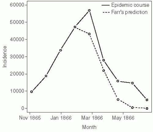 Figure 6-1 Epidemic course of an 1865-1866 epidemic of cattle plague in England compared with predictions using William Farr’s “assumption of the second ratio” (first predicted date is February 24, 1866). Data from Brownlee J. Historical Note on Farr’s Theory of the Epidemic. British Medical Journal 1915;2(2850):250-2. |
Arthur Ransome was perhaps the first to articulate what is one of the most important principles of infectious disease dynamics: that the depletion of susceptible individuals in the population can cause an epidemic to recede, even if not everyone in the population has been infected.4 In doing so, he anticipated modern efforts to use the principles of infectious disease dynamics to understand and predict epidemics much as we do the weather: “Like the cyclones of the atmosphere, these storms of disease can only be tracked, and the laws of their course discovered, by the combined efforts of many observers.”4 Ransome developed his ideas on the importance of susceptible dynamics and postulated that multiyear cycles in epidemics are likely the result of an accumulated density of susceptible individuals through births over time.5
While Ransome recognized the important role played by susceptible hosts in epidemic dynamics, he never developed a precise mathematical formulation of his hypothesis. Perhaps the first to do so was a Russian physician, Pyotr Dimitrievich En’ko,6 who presented his model in an 1889 paper, “On the course of epidemics of some infectious diseases.”7 En’ko’s model is similar to one later developed by Lowell Reed and Wade Hampton Frost (discussed later in this section), calculating the number of infectious cases expected to occur in a generation of an epidemic based on the probability of members of the current susceptible population making contact with a member of the current infectious population.7 En’ko used his model to model the course of epidemics and was one of the first to observe that there exists a density of susceptible individuals below which an epidemic will not occur. Despite the importance of En’ko’s model, it did not gain wide adoption until Reed and Frost’s formulation was popularized in the 20th century.
Separately, Ronald Ross, a British medical doctor with a strong interest and aptitude in mathematics, was working in India to understand the transmission of malaria.8 Ross received the Nobel Prize for his discovery that mosquitoes transmit malaria. Subsequent to this discovery, Ross developed a model of malaria transmission that would lay the foundation for decades of malaria research and for mechanistic descriptions of contagion. Using this model, he identified thresholds of mosquito populations below which transmission of malaria would not be sustained. Ross argued that mosquito control could eliminate malaria transmission—a position that many of his contemporaries rejected, as they believed that mosquito populations of even very small numbers could continue to sustain transmission. Decades after Ross’s work, MacDonald used his framework to advocate for mosquito control when effective insecticides were available and public health authorities were considering large-scale malaria control efforts.9
Wade Hampton Frost was a professor of epidemiology and Lowell Reed was a professor of biostatistics at the Johns Hopkins School of Public Health, and both eventually went on to serve as deans of the School of Public Health. Frost and Reed developed and refined a statistical model of epidemics similar to that developed by Pyotr En’ko that considered a series of distinct generations of
infection. Under the Reed-Frost model, the number of cases seen in a generation is calculated as follows:10
infection. Under the Reed-Frost model, the number of cases seen in a generation is calculated as follows:10
where Ct is the number of new cases occurring in generation t, St is the number of individuals that remains susceptible to infection in generation t, q = 1 — p is the probability that a susceptible individual avoids contact with any given case (p is the probability of such a contact), and qct is the probability that a susceptible individual avoids infectious contact with all Ct infectious cases. Reed and Frost predominantly used their model as a teaching tool, but it was resurrected and popularized by other authors. Reed and Frost were also responsible for what may be the first epidemic simulator. Created before the computer era, this mechanical device used small beads to represent individuals and could be used to simulate stochastic epidemics.11 The chain binomial models of En’ko and Reed and Frost are the foundation of analysis of transmission and intervention effects in households, schools, and other tightly interacting social units.12
Another thread of scientific development that helped lay the foundation for much of modern infectious disease dynamics focused on the use of mass-action kinetics to describe the interactions of infectious and susceptible individuals. Here Ronald Ross again played a central role. Ross supervised Anderson Gray McKendrick, a Scottish physician, during an antimalarial campaign in Sierra Leone. At this time, Ross introduced McKendrick to his model of malaria and encouraged McKendrick to extend his work. McKendrick used ideas from chemical reaction kinetics to formulate a model of transmission that treats the interaction of susceptible and infectious individuals as similar to the collision of molecules.13 He published a model that represented transmission dynamics as a compartmental model expressed as continuous time ordinary differential equations.14 Later, McKendrick worked with William Ogilvy Kermack, a chemist by training, to develop this model and identify key conclusions, including the critical density of susceptible persons needed for an epidemic to propagate.15
Since the early 20th century, there has been an ever-growing interest in infectious disease dynamics. The history and main ideas developed during this period have been reviewed in many excellent texts, including, in no particular order, those by Anderson and May (1991);16 Dietz (1975);17 Bailey (1957, 1975);18, 19 Keeling and Rohani (2007);20 Halloran (2010);12 and Heesterbeek (2005).13 We refer the reader to these texts for a more detailed review of the history of ideas in this field.
DETERMINANTS OF EPIDEMIC GROWTH
The rate at which an epidemic grows (or recedes) is determined by the number of infections that occur in each successive generation of pathogen transmission and the time between these generations. These two quantities, which are referred to as the reproductive number and the generation time, respectively, form the basis for much of our thinking about the dynamics of the epidemic process.
The Reproductive Number
The reproductive number, R, is the number of secondary cases expected to be caused by a single, typical infected individual in a population with some level of susceptibility. If the population is fully susceptible, this is termed the basic reproductive number and denoted as R0 (estimates of R0 for some common disease are shown in Table 6-1). The reproductive number is the primary metric used to quantify the transmission of a disease in infectious disease dynamics; it provides a measure of how fast an outbreak will grow across subsequent generations of transmission. For instance, for influenza R0 ≈ 2; hence we would expect a single infected case to cause 2 cases after one generation, 4 cases after two generations, 8 cases after three generations, and so on. For measles, where R0 ≈ 11, we would expect to see 11 cases in one generation, 121 cases in two generations, and 1331 cases in three generations. However, the observed speed of growth does not depend only on R0, as the average time between generations of transmission varies by disease (see the discussion of generation time in the next subsection) and the number of people available to be infected decreases over time as the pool of susceptible individuals is depleted by infection.
While R0 refers to the number of cases caused by a typical individual in a completely susceptible population, R refers to the number of cases caused by a typical infectious individual given the proportion of individuals still available to be infected at the current time. R changes over time and is sometimes denoted Rt, whereas R0 refers to a theoretical time 0 when the entire population is susceptible. R accounts for the reduction in transmission due to some individuals being immune (Figure 6-2). For instance, if R0 is 4, but half of a primary case’s contacts are immune due to previous infection or vaccination, then we would expect
that case to infect only 2 individuals; in this scenario, R would be equal to 2. In general, if st is the proportion of the population still susceptible to infection at time t, then Rt is R0st.
that case to infect only 2 individuals; in this scenario, R would be equal to 2. In general, if st is the proportion of the population still susceptible to infection at time t, then Rt is R0st.
Table 6-1 R0 for Multiple Pathogens | ||||||||||||||||||||||||||||||
|---|---|---|---|---|---|---|---|---|---|---|---|---|---|---|---|---|---|---|---|---|---|---|---|---|---|---|---|---|---|---|
| ||||||||||||||||||||||||||||||
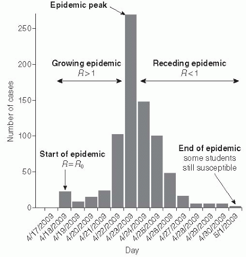 Figure 6-2 Dynamics of an emergent influenza epidemic. Adapted from Lessler J, Reich NG, Cummings D a T, et al. Outbreak of 2009 pandemic influenza A (H1N1) at a New York City school. New England Journal of Medicine. 2009;361(27):2621. |
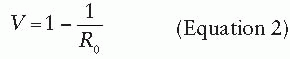
When R is less than 1, then the infectious individuals will no longer replace themselves; that is, there will be fewer infectious individuals in the current generation than in the previous generation. At this point the epidemic will begin to wane and eventually die out. Likewise, when R is less than 1 in a population, introduction of a disease will not cause a widespread epidemic—a state usually referred to as herd immunity. When a population has herd immunity against a disease (R < 1), it is protected from sustained transmission of the disease (note that herd immunity is also used to refer to the protection that susceptible individuals in the population get from the immunity of others, even when R is greater than 1). Because of the relationship between susceptibility and R(R = R0s), we can derive an expression for the proportion of the population that must be immune for herd immunity to occur. In other words, we can determine the proportion of the population that must be successfully vaccinated to induce herd immunity: the critical vaccination threshold V. Based on the previously discussed relation, it follows that:
The role of vaccination in inducing herd immunity will be discussed in more detail with specific reference to rubella later in this chapter.
R0 and R depend on both the pathogen and the setting. Table 6-1 shows some typical estimates of the basic reproductive number for multiple pathogens. Estimates vary considerably by pathogen, but we emphasize that they also vary from setting to setting. Setting-to-setting variability results from aspects of the transmission process that vary between locations, including environmental characteristics,
crowding, underlying health status of the population, and cultural factors that affect the rate at which individuals make potentially infectious contacts.
crowding, underlying health status of the population, and cultural factors that affect the rate at which individuals make potentially infectious contacts.
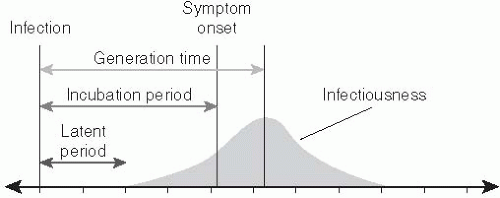 Figure 6-3 Schematic of an infected individual’s progression in relation to time of infection. Gray indicates infectiousness over time. Incubation period is defined by the time from infection to symptom onset. The latent period is defined by the time from infection to non-zero infectiousness. The generation time is the mean time from infection to time of infection in those individuals that this person infects. We expect this to be equal to the latent period plus the time from the start of non-zero infectiousness to the probability weighted center of the infectiousness distribution. |
The inclusion of the word “typical” in the definition of the basic reproductive number admits the possibility that infectiousness across individuals may be heterogeneous. The basic reproductive number is the average number of secondary infections created by a single infectious individual in an entirely susceptible population, averaging over all types of individuals who may be first infections in a population.
Generation Time
The generation time (or generation interval) of an infectious disease is the time separating the onset of infection in an individual (the infector) and the time that person transmits to another individual (the infectee). While the reproductive number dictates the number of infections produced by each generation of transmission, the generation time specifies a time scale at which these transmissions accumulate. The generation time is also referred to as the serial interval, a term coined by Hope-Simpson that is often used to refer to the time between symptom onset in successive generations of infection.21** The generation time is not fully observable, as the precise moment of infection is difficult, if not impossible, to detect.
A proxy that is often used to estimate the generation time is the time separating the onset of symptoms in infector and infectee (i.e., the serial interval). Two other time periods—the latent period and the infectious period—also affect the generation time. The latent period is the time between infection and the onset of infectiousness. The infectious period is the duration of time for which individuals are infectious. The infectiousness of individuals may vary over the infectious period. The mean generation time can be approximated by the mean latent period plus the time until the center of the infectious period weighted by transmissibility (Figure 6-3).
ELEMENTS OF THE COURSE OF INFECTION
The course of infection within individuals has its own dynamics, which need to be well characterized for a full description of the dynamic disease process. While the within-host disease process has been modeled at varying degrees of complexity, the distribution of three time periods characterize the essentials of the infectious process: the incubation, latent, and infectious periods.
Incubation Period
The incubation period is the time between infection with a disease and the development of symptoms (see Figure 6-3). It plays an important role in the dynamics of disease transmission because it dictates when cases will be detected relative to individuals’ time of infection. This delay must be accounted for when determining the true infectious burden and evaluating the effect of control measures based on symptomatic surveillance.22
While statements of a mean incubation period or range for the incubation period are common in the infectious disease literature, they are often too vague for use in dynamic models of disease transmission.23 Typically, in dynamic models, incubation periods are assumed to follow some statistical distribution. Common choices for this distribution are exponential, log-normal, Weibull, and gamma distributions.24, 25
Latent Period
The latent period is the time between when an individual is infected and when he or she becomes infectious (see Figure 6-3). While in some cases the latent period and the incubation period have the same length, for many diseases this is not the case. Perhaps the most dramatic example of such a discrepancy involves HIV/AIDS, for which the incubation period can last years longer than the latent period. Care should be taken when reading the literature, as not all authors are precise in distinguishing the incubation period from the latent period, often referring to the latter as the former.
When exploring the dynamics of epidemics, it is usually the latent period, rather than the incubation period, in which we are interested because the latent period has the more profound effect on the generation time, and hence epidemic growth. However, the incubation period may also be important, especially when attempting to interpret observed case counts, which may not include all infections that have already occurred.
The distinction between the incubation period and the latent period is especially important when evaluating the effect of control methods based on symptomatic surveillance. If infectiousness proceeds symptom onset (i.e., the latent period is shorter than the incubation period), as in HIV, then interventions based on targeted controls toward symptomatic individuals are unlikely to be effective.26 Diseases where symptom onset is coincident with, or even proceeds, infectiousness (e.g., smallpox) are more likely to be controlled using methods based on symptomatic surveillance. Hence, the proportion of transmission that takes place before the onset of symptoms may be an important metric of controllability.26
As with the incubation period, the latent period is usually modeled as following an exponential, lognormal, Weibull, or gamma distribution.
Infectious Period
The infectious period is clearly one of the most important determinants of infectious disease dynamics. The infectious period for an infection can range from days (e.g., influenza) to years (e.g., HIV) and plays an important role in determining the reproductive number for that disease. Even a difficult-to-transmit infection may cause a large number of secondary cases if individuals remain infectious for a long period of time. For instance, HIV has a fairly low per-act probability of transmission (0.001 per heterosexual act, 0.008 per male-homosexual act),27, 28 but individuals remain infectious for years, leading to a relatively high basic reproductive number (2-5).26 In contrast, measles has a comparatively short infectious period (approximately 1 week)29 but is highly infectious during that period and has a very high basic reproductive number (7 to over 20, see Table 6-1).
The dynamic effects of infectious disease control measures are often best understood by considering their effects on the infectious period. The primary effect of treatment, in terms of epidemic dynamics, is to decrease the infectious period. Similarly, case isolation can be seen as decreasing the effective infectious period of those isolated. In some circumstances a treatment may increase the infectious period—for instance, supportive care that prevents death but does nothing to prevent transmission.
The infectious and latent periods play a primary role in determining the generation time of an infection. If infectiousness in evenly distributed across the infectious period, then the mean generation time will be equal to the mean latent period plus one-half the mean infectious period. In general, infectiousness may not be uniform during the infectious period, though the mean timing of infection may still be determined through more sophisticated techniques (see Carrat et al.’s work for an example).30
DYNAMIC MODELS OF THE EPIDEMIC PROCESS
As stated previously, the reproductive number is the product of the basic reproductive number and the susceptible fraction. A central challenge of infectious disease dynamics is to describe the dynamics of transmission given changes in the susceptible and infectious populations. Compartmental models provide a method to integrate our understanding of the constituent parts of disease transmission and the course of infection into dynamic models of the epidemic process.
Compartmental Models
In compartmental models, each individual in the population exists within a compartment (or state) based on that person’s current role in the transmission process. For immunizing infections (i.e., those that induce a protective immune response), compartmental models usually consist of (at least) compartments for individuals who are susceptible to infection (the S compartment), infectious (the I compartment), or recovered and immune from further infection (the R compartment). This last compartment can also be thought of as consisting of all those individuals who have been removed from the infectious dynamics in the population, which explains why it is sometimes referred to as the removed compartment. The state of the model at any given point in time is the number
of individuals who reside in each of the model compartments. For mathematical clarity, the population is usually considered to be continuous; hence partial individuals may reside in any particular compartment.
of individuals who reside in each of the model compartments. For mathematical clarity, the population is usually considered to be continuous; hence partial individuals may reside in any particular compartment.
In simple compartmental models, the compartments in the model are usually listed in the order in which individuals travel through them. For example, a model in which susceptible individuals become infectious and then recover is an SIR model, one in which recovered individuals can eventually lose immunity and become susceptible again is an SIRS model, and one in which individuals reside in an exposed but not yet infectious compartment during their latent period (the E compartment) is referred to as an SEIR model. Figure 6-4 provides examples of some compartmental model structures.
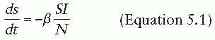
The dynamics of an infection in a population is defined by the rate at which members of the population move between compartments. In some cases, this rate will be dictated by the biology of the disease process—for instance, the rate at which individuals recover, moving from the I compartment to the R compartment. In other cases, the rate will depend on the state of the population—for instance, the rate at which susceptible individuals become infectious (i.e., move from the S compartment to the I compartment) is driven by the number of infectious individuals in the population. The rates at which individuals transition between compartments define a set of differential equations that capture the epidemic dynamics of the disease (under a set of assumptions to be discussed later). For instance, a basic SIR model can be defined by the following set of equations:
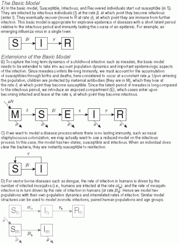 Figure 6-4 Examples of important types of compartmental models. |
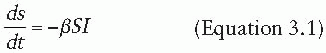
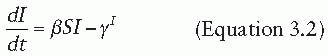
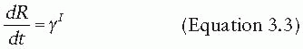
That is, susceptible individuals become infected at rate βI, at which point they instantly become infectious. Infectious individuals remain infectious for an average of 1/γ days (i.e., they recover at the rate of γ), at which point they recover and are permanently immune. In this formulation, the transmission coefficient, β, combines the contact process by which the disease spreads with the per-contact infectiousness of the disease considered. The product of the number of susceptible and infectious individuals in the population (S • I) represents all of the potential infectious contacts between infectious and susceptible individuals in this population. Hence, the parameter β is the probability that a potential infectious contact actually occurs and that the contact results in an infection. What constitutes an “infectious contact” varies by disease and setting, in some cases requiring direct person-to-person contact (e.g., for Ebola virus), and in others representing contamination and subsequent contact with some environmental reservoir (e.g., hepatitis A contamination of a salad bar). When the contact process is well understood, it is often useful to break β into its constituent parts: the rate at which potentially infectious contacts are made and the proportion of those contacts that result in infection. This formulation is particularly useful when describing sexually transmitted infections.
Force of Infection
An important metric of the infection pressure that susceptible individuals experience is the force (or hazard) of infection. The force of infection is the rate at which susceptible individuals acquire infection at a particular time, regardless of the source. In other words, it is the total hazard a susceptible individual encounters given all exposures to infectious individuals. In the basic SIR model, the force of infection is βI. The force of infection is often easier to estimate from empirical data than the basic reproductive number, as it can be directly estimated from longitudinal data on infection status for a cohort of susceptible individuals without any information on the size of the infectious population. Estimation of the force of infection can be an intermediate step in estimating the basic reproductive number and other parameters describing epidemic dynamics.
Transmission Rates: Density and Frequency Dependent Transmission
In the basic SIR model presented earlier (Equations 3.1, 3.2 and 3.3), we assume that susceptible individuals become infected at a rate that is directly proportional to the number of infectious individuals, βI. Under this formulation, the basic reproductive number is the product of the transmission coefficient (β), the length of infectiousness (γ), and the total population size (N):
Under this formulation, R0 is not consistent in populations of differing sizes if β is assumed to be constant. For example, a disease for which R0 is 2 in a population of 10,000 individuals would fail to spread in a population of 4000 (R0 = 0.8), but would demonstrate far more explosive spread in a population of 100,000 individuals (R0 = 20). Models like those defined by equations 3.1, 3.2 and 3.3 are called “density-dependent” models because they suggest that members of a population existing in a fixed area all come in contact with one another no matter how many individuals are present in the population. Thus it is assumed that the rate at which contacts are made scales with density, such that all members of a population of 100,000 have contact with one another just as a population of 10 would. Hence, the disease will spread more effectively in larger populations. In many cases, this outcome makes intuitive sense, especially for pathogens in animal and plant populations where the frequency of contact with individuals of the same species may be driven predominantly by population density.
However, empirical evidence for infectious diseases in humans suggests that R0 is surprisingly consistent across a variety of contexts. Estimates of the basic reproductive number for the 2009 pandemic involving H1N1 influenza ranged from 1.2 to approximately 3.31, 32 and 33 Despite a 20-fold difference in population density, similar reproductive number estimates were obtained for New Zealand (1.9) and Japan (2.3).32, 33 This consistency is not completely surprising given the contexts in which most close human interactions take place. Whether in Manhattan or rural Wyoming, most households in the United States contain between 1 and 5 individuals, and even across the entire world, variation in household size will be less than variation in total population density. Workplaces, restaurants, and entertainment venues will fall within a similarly narrow range of sizes. Because the density dependence assumption often appears not to hold, an alternative “frequency dependent” formulation of the SIR model is often used:
In the frequency-dependent formulation, the interpretation of the transmission coefficient changes. The term S/N is the probability that any random contact that someone in I makes will be with someone susceptible to infection. The transmission coefficient β now combines the number of contacts that I is expected to make during a single time step and the probability a contact results in a new infection (note that β in the two models has different units). Under this formulation, the expression for the basic reproductive number becomes:
which is invariant to the size of the population. Similarly, the epidemic dynamic from a frequency dependent model is the same when expressed as a percentage of the population regardless of the size of the population.
HOST POPULATION STRUCTURE
Homogeneous Mixing
One critical assumption of compartmental models is that of homogenous mixing. In these models, we assume that populations behave similarly to how a gas behaves in a container: people move about randomly and have an equal probability of contacting any member of the population of a particular type. For instance, in a simple SIR model every infectious individual has an equal probability of coming into contact with every susceptible individual (i.e., there is no clustering, hyperinfectivity, or other type of aggregation influence). Human populations are highly structured, and homogenous mixing is clearly an over-simplification; nevertheless, over some scales, models built on this assumption can accurately model epidemic data.34, 35
Introducing Structure
Thus far we have assumed that all individuals in the same disease state are identical. In reality, important heterogeneities exist between individuals that can affect the dynamics of transmission. It is possible to relax the assumption of identical, homogenously mixing individuals by introducing additional model compartments and specifying transmission coefficients based on the interactions between these compartments.
Age
Age can alter a person’s risk of acquiring and transmitting an infectious disease through multiple pathways. For example, young individuals may be protected by maternal antibodies or have increased susceptibility because of immaturity of their immune response. Infectious contacts that might transmit respiratory and gastrointestinal infections may occur at increased rates among young individuals because of reduced hygienic practices. Age has been shown to be a predictor of whom individuals have social contact with, with the age distribution of contacts showing a strong tendency for contacts to occur between individuals of a similar age, but also reflecting family structure.36 Models that incorporate this heterogeneity may exhibit fundamentally different behavior than models that do not. In addition, age dictates the timing of immunization targeting many pathogens. Models that incorporate age structure can compare multiple alternative age-specific immunization programs.
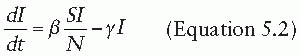
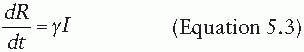
Age is often modeled by adding age-specific compartments for each disease state and specifying transmission coefficients capturing the rates at which members of these age compartments interact.37, 38 and 39 For example, consider the model shown in Figure 6-5, which divides the population into three groups: preschoolers, school-aged children, and adults. Each of these groups has a different level of interaction both within their group and with people in other groups. School-aged children might have the most interaction among themselves (β22 > β11, β33, but the least interaction with preschoolers or adults. Preschool-aged children, in contrast, may interact less among themselves than school-aged children do (β11 < β22), but likely have a closer relationship to adults (β13 > β23). For many questions and diseases, the use of models with population structure is critical, as important heterogeneities might change our conclusions about the effectiveness of interventions and other factors (see the example of rubella later in this chapter).
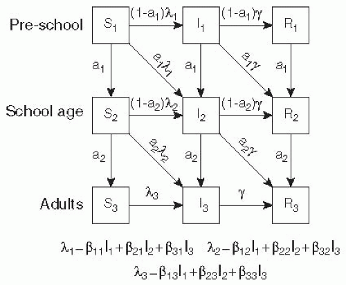 Figure 6-5 A simple age structured SIR model where individuals move through (1) pre-school, (2) school aged and (3) adult categories. |
The average age of infection can be derived from compartmental models and expressed as a function of model parameters. Empirical data on the average age of incident cases can be used to parameterize these models and obtain estimates of the basic reproductive number.16 With certain assumptions about the demographic structure of the population, the basic reproductive number is related to the average age of infection by the following expression:
where L is the average life expectancy of individuals in the population.
Gender
Sexually transmitted infections may be transmitted asymmetrically with respect to gender, with different rates of transmission being noted from women to men, men to women, men to men, and women to women. Rates of sexual partnership may vary across these different types of couplings in any population. Models of sexually transmitted infections (STIs) introduce host heterogeneity to account for these differences in contact rates and transmission rates. Models of STIs among exclusively heterosexual couples are similar in structure to models of vector-borne diseases where each host transmits the disease exclusively to the other host type. A key challenge in crafting models of STIs with multiple genders and types of partnerships is to balance partnerships across genders. Reconciling empirical data on partnership formation in a way that balances sexual contacts made by each group is often difficult and may require reinterpretation of empirical data.
When host heterogeneities are present, the individual basic reproductive numbers within each age group bounds the overall basic reproductive number, but this quantity must be estimated while accounting for the typical infective individual in the population. Later in this chapter, we present methods to estimate the basic reproductive number from models with structured host populations.
Agent/Networks
One of the key assumptions of compartmental models of infectious disease is that all individuals within the population, or within subpopulations, have the same chance of having an infectious contact with other individuals within that population. This is never truly the case, but for many diseases transmitted by person-toperson contact (e.g., measles, rubella), this assumption is close enough to reality to give accurate predictions. However, for some diseases, particularly STIs, individual variations in contact may have a profound effect on disease dynamics. Furthermore, even in the cases of constant contact probability, the specifics of how contact occurs may be important to disease dynamics. For instance, “concurrent” contacts in STIs can greatly increase the speed of disease spread and population risk.40
One approach to dealing with heterogeneities in contact, as well as other types of heterogeneity (e.g., differences in host susceptibility), is to explicitly model each individual in the population and his or her infection status. In network models, individuals are depicted as nodes in a network of potentially infectious connections. In agent-based models, individuals are depicted as “agents” that exist in some virtual environment where they contact (or do not contact) other agents based on some set of behaviors. These definitions are somewhat malleable, and the distinction between the two approaches is not always clear. Agent-based models typically incorporate some process by which agents can gather and interpret information on the state of other agents in the model.41 For example, in dynamic network models, contacts between nodes (i.e., agents) may change based on some set of rules analogous to agent behaviors.41 In both approaches, individuals are considered to have a disease state (analogous to the compartmental model states), such as “susceptible,” “infectious,” or “immune.” Individual-based approaches, however, allow for an expansion of the state space to include subtle differences between infected hosts; for example, each host may have a different transmission probability to those around the host.
Agent-based models have been built at a variety of spatial scales, from single hospital unit up to entire countries,42, 43 and 44 and have played a particularly important role in pandemic preparedness planning. Network-based models have proved particularly useful in modeling the transmission of STIs, where contact networks tend to be heterogeneous, and their structure can play an important role in epidemic dynamics.45
Network- and agent-based models are intuitively appealing because they can, in theory, represent almost any level of realism and complexity in the disease transmission process. However, this power and flexibility come at a cost. Greater realism generally requires more background information or assumptions about host behavior and the disease process. The number of assumptions needed often makes it difficult to directly estimate model parameters from a disease process or to perform adequate sensitivity analyses of the results. Furthermore, it is easy to embed arbitrary structural assumptions in agent-based models that are difficult to communicate to other researchers or to replicate, which in turn may make replication, comparison, and generalizable inferences challenging. Despite these caveats, agent-based and
network-based approaches remain powerful methods to model dynamic disease processes, and are often the only tool flexible enough to handle certain problems.
network-based approaches remain powerful methods to model dynamic disease processes, and are often the only tool flexible enough to handle certain problems.
Box 6-1 Modeling Methodologies
Branching Processes
Basic branching processes assume that infection occurs in discrete non-overlapping, overlapping generations. The number of infections in each generation is a function of the number of infections in the previous generation times the reproduction number, R.
Model Inputs
Branching models assume a known distribution of “child” infections for each “parent” infection occurring in the previous generation. In their simplest form, this is simply R.
Compartmental Models
Compartmental models divide the population into “compartments” based on infectious state and demographics—for example, the S compartment for susceptible individuals and the I compartment for infectious individuals. At any given time, the state of the population is defined by the number of people in each compartment. It is assumed that the population is homogeneous within each compartment (i.e., an individual in the population is fully defined by his or her compartment) and that homogeneous mixing occurs between compartments.
Model Inputs
In general, a transmission coefficient and the average time that individuals remain infectious must be specified. More complex models may require the length of the latent period (SEIR models), birth and death rates (open population models), and seasonal variations in the transmission coefficient to be known. The number of parameters that must be specified generally scales with the number of compartments modeled.
Network- and Agent-Based Models
Network- and agent-based models explicitly represent each individual in the population and his or her potentially infectious contacts. These contacts may be represented by a static or a dynamic network structure (network-based models) or may be the result of an individual’s changing status and behavior over time (agent-based models). These models make few assumptions other than that the specification of the model capture the important aspects of the infectious process.
Model Inputs
Network- and agent-based models often require a large amount of information about the population, although simplified models can be sometimes revealing. In addition to disease natural history (e.g., latent and infectious periods) and per-contact infection probabilities, it is often necessary to know the population distribution of contact patterns, the daily movements and other behaviors of the members in the population, and the way in which population members of different types are distributed across geographic space.
TYPES OF PATHOGENS
There is huge diversity in the types of pathogens that cause infectious disease. In terms of epidemic dynamics, two differences are of primary importance: (1) how the pathogen induces (or does not induce) host immunity and whether this affects future transmission, and (2) how the pathogen is transmitted between hosts.
Immune Status and Pathogen Population Structure
In the simplest formulation, hosts are born susceptible, then are infected, and then recover and are forever immune to future infection. Although there are few diseases for which this simple formulation is completely true, depending on the question of interest such a simplified structure may be adequate to capture the essential disease dynamics. For instance, while the period of maternal protection to measles may be very important for setting vaccine policy, it is unimportant in predicting the course of a measles outbreak in a measles-naive population. While in many cases it may be necessary to develop a disease-specific immune model, most diseases fall into one of the following major classes.
Pathogens Conferring Lifelong Immunity (SIR, SEIR)
Pathogens such as measles, smallpox, and rubella confer lifelong immunity to future infection. For these diseases, a simple susceptible-infected-recovered (SIR) model is usually adequate to capture the epidemic
dynamics (Figure 6-4A). Even when full immunity is temporary (e.g., cholera), models that assume full immunity after infection are adequate for capturing the dynamics at shorter time scales (e.g., over the course of a single epidemic).
dynamics (Figure 6-4A). Even when full immunity is temporary (e.g., cholera), models that assume full immunity after infection are adequate for capturing the dynamics at shorter time scales (e.g., over the course of a single epidemic).
Pathogens with Protective Maternal Antibodies (MSIR, MSEIR)
Many diseases are characterized by a period following birth where infants are immune to infection due to the presence of maternal antibodies transplacentally transferred from mother to infant.46 This phenomenon can have important implications for disease dynamics, especially for diseases such as measles, where the presence of maternal antibodies interferes with the action of vaccines.47 When maternal antibodies are important, a maternally immune (M) compartment is usually added to models to account for the period of maternal protection (and possible reduced vaccine efficacy) (Figure 6-4B).
Pathogens Conferring No Immunity (SIS)
Some pathogens, particularly some bacterial infections, confer no significant immunity even within the course of a single epidemic. In these cases, a susceptible-infectious-susceptible (SIS) model, in which individuals immediately return to the susceptible compartment after treatment or recovery, is appropriate (Figure 6-4C). The reasons for continued immunity vary. In some cases (e.g., cutaneous Staphylococcus infection), the host mounts no permanent immune response; in others, the diversity of pathogen strains is such that individuals are effectively susceptible to another infection with a different strain immediately after recovery.
Pathogens Conferring Temporary or Waning Immunity (SIRS)
In some cases, a pathogen may induce temporary immunity but this immunity may wane eventually, making a susceptible-infectious-recovered-susceptible (SIRS) model appropriate. The reasons for returning susceptibility vary between pathogens. In the case of influenza, an SIRS model allows epidemiologists to approximate the effect of the influenza virus changing over time through the process of antigenic drift, eventually becoming different enough that individuals are no longer are immune to the circulating virus.46 In contrast, cholera immunity is temporary not because of a changing bacterium but due to a waning in host immunity itself,48 yet an SIRS model is still appropriate. In many cases, a pathogen that is truly SIRS can be modeled as SIR (if we are interested in only a single epidemic) or as SIS (if the period of immunity is insignificant on the timescale being studied).
Pathogens Conferring Partial Immunity or Cross-Immunity Between Strains
In some cases, an individual’s immune status and infection history must be modeled in more detail than is captured by a single compartment. This is often true when infection confers partial immunity to future infections with the same pathogen (for instance, protecting against systemic disease) or when multiple pathogen strains exist that provide partial protection between one another. There are also cases, such as dengue, where previous infection increases the probability of severe disease in a subsequent infection. Modeling these systems can be quite complex, requiring a large number of susceptible, infectious, and recovered compartments.
Figure 6-6 shows a simplified model of a denguelike system with two strains. Infection with one strain gives immunity to that strain, but individuals remain susceptible to the other strain. After infection with both strains, individuals are immune to all future infection.
Mode of Transmission
Direct Contact
The default assumption of most of the models presented so far is that infection is primarily transmitted by direct contact. Even within the range of what are considered directly transmitted infections, however, there can be a range of contact types. For instance, influenza may be transmitted by touch, by small droplet particles that travel some distance in the air, and by pathogens being deposited on surfaces (i.e., fomites).49 In most models, the combined effect of all of these modes of transmission are collapsed into a single β term, which encompasses both the probability of each type of contact occurring and the probability of successful transmission if it does occur. In other models, particular modes of contact are considered independently, as in explicit modeling of fomite-mediated transmission.50
Related posts:

Stay updated, free articles. Join our Telegram channel

Full access? Get Clinical Tree


