The disciplines of epidemiology and biostatistics apply to gynecologic oncology in defining cancer occurrence and survival, identifying risk factors, and implementing strategies for treatment or prevention, including the proper design of clinical trials. Epidemiology and biostatistics are essential to the practice of evidence-based medicine. Some key principles of epidemiology and biostatistics are considered under the headings of descriptive statistics, etiologic studies, statistical inference and validity, and cancer risk and prevention. Standard statistical and epidemiologic texts present more detailed discussions and computational formulas (1,2).
Descriptive Statistics
Cancer is described in populations by statistics related to its occurrence and patient survival. How cancer varies by age, ethnicity, and geography is of particular interest. Descriptive statistics about cancer in the United States can be obtained from the National Cancer Institute through its Web site: http://www.seer.cancer.gov/. Descriptive statistics about cancer in the world can be obtained from the International Agency for Research on Cancer through its Web site: http://www-dep.iarc.fr/.
Incidence
The incidence rate (IR) is defined as the number of new cases of disease in a population within a specified time period:
IR = New cases/Person-time
The fact that time is a component of the denominator should help clinicians avoid the misapplication of this term to prevalence—another measure of disease occurrence that includes both old and new cases existing at a single point in time.
Cancer Incidence and Mortality
Cancer incidence or mortality is usually stated as cases (or deaths) per 100,000 people per year, or as cases per 100,000 person-years. Incidence or mortality is measured in a specific population over a specific period. For example, country or state cancer registries count the number of new cancer cases diagnosed or cancer deaths among residents over a year, and divide that figure by census estimates of the total population in the region.
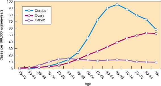
Figure 6.1 Age-specific incidence curves for gynecologic cancers in women in the United States, 2006–2010. (Modified from Howlader N, Noone AM, Krapcho M, et al., eds. SEER Cancer Statistics Review, 1975–2010. Bethesda, MD: National Cancer Institute. Available at http://seer.cancer.gov/csr/1975_2010/. Based on November 2012 SEER data submission, posted to the SEER web site, 2013.)
Crude Incidence or Mortality
Crude incidence or mortality is the total number of new cancers (or deaths) that occur over a specified time in the entire population.
Age-specific Incidence or Mortality
Age-specific incidence (or mortality) is the number of new cancers (or deaths) that occur over a specified time among individuals of a particular age group divided by the total population in that same age group. Age-specific incidence or mortality rates are the best way to describe the occurrence of cancer in a population and are commonly graphed in 5- or 10-year groups. Annual age-specific incidence and mortality curves for the common malignant gynecologic cancers in the United States based on all women in the Surveillance, Epidemiology, and End Results (SEER) survey area for 2006 to 2010 are shown in Figures 6.1 and 6.2 (3). Invasive cervical cancer shows a gradual rise and plateau after 40 years of age at approximately 15 cases per 100,000 women-years. Cancer of the corpus (largely endometrium) rises during the perimenopause and peaks at approximately 90 cases per 100,000 women-years after 60 years of age. Cancer of the ovary displays an increase during the perimenopause and peaks after 70 years of age at approximately 50 cases per 100,000 women-years. In situ cervical intraepithelial neoplasias (CIN) are no longer being tabulated by the SEER registries. The vast majority of these cases are seen between the ages of 20 and 50 years, with a peak occurrence of approximately 200 cases per 100,000 women per year at ages 25 to 29. In addition, SEER is no longer counting ovarian tumors of borderline malignancy, accounting for a decline of 21% in incidence and 6% in mortality between 2004 and 2006.
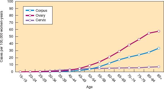
Figure 6.2 Age-specific mortality curves for gynecologic cancers in women in the United States, 2006–2010. (Modified from Howlader N, Noone AM, Krapcho M, et al., eds. SEER Cancer Statistics Review, 1975–2010. Bethesda, MD: National Cancer Institute. Available at http://seer.cancer.gov/csr/1975_2010/. Based on November 2012 SEER data submission, posted to the SEER web site, 2013.)
Table 6.1 Lifetime Risk of Acquiring or Dying from Gynecologic Cancers in White and Black U.S. Womena

Cumulative Incidence or Mortality
Cumulative incidence (or mortality) may be thought of as the proportion of people who develop disease (or die from it) during some period of observation. Cumulative “incidence” is technically a misnomer because it does not contain time in the denominator but, rather, is expressed as a percentage.
The cumulative IR (CIR) may be crudely approximated from age-specific IRs by the following formula:
CIR = ∑IRi(ΔTi)
where IRi is the age-specific rate for the i age stratum and ΔTi is the size of the age interval of the i stratum (usually 5 years).
Cumulative incidence, summed over the age range 0 to 85 years, yields the “lifetime risk” for cancer occurrence or death. Lifetime risks that a woman in the United States will have or die from cancer of the cervix, corpus, or ovary are shown in Table 6.1 and confirm that a US woman has a greater risk of developing cancer of the corpus than cervical or ovarian cancer, but a higher risk of dying from ovarian cancer than cervical or endometrial cancer combined.
Age-adjusted Incidence or Mortality
Age-adjusted incidence (AAI) or mortality is obtained by summing weighted averages of the incidence or mortality rates for each age stratum. The weight is derived from the age distribution of a standard population:

where IRi is the IR in the i age stratum, and Wi is the number of people in the i stratum in the standard population.
Age-adjusted rates are better than crude rates for summarizing incidence or mortality when comparing cancer occurrence among populations that may differ in their age structure. An “old” population would have a higher crude incidence of ovarian cancer and a lower crude incidence of carcinoma in situ of the cervix than a “young” population, even though both populations might have identical age-specific incidences for each disease. Cancer rates adjusted to the “world population standard” are shown in Table 6.2.
Worldwide, cervical cancer is the most prevelant of the gynecologic cancers and is second only to breast cancer in overall occurrence. Cervical cancer is most frequent in southern Africa and Central America and least frequent in North America and parts of Asia. Cancer of the corpus is least frequent in Africa and Asia and most frequent in North America. Ovarian cancer is least frequent in Africa and Asia and most frequent in northern Europe.
Table 6.2 Age-adjusted Incidence Rate for the Gynecologic Cancers in Comparison with Other Major Cancers in Women in 2008a

Prevalence
Prevalence (P) is the proportion of people who have a particular disease or condition at a specified time. Prevalence can be calculated by multiplying incidence times the average duration of disease:
Prevalence = Incidence × Average duration of disease
More commonly, prevalence is derived from cross-sectional studies in which the number of individuals alive with a particular condition is identified from a survey and stated as a percentage of the total number of people who responded to the survey. Other examples of studies that yield prevalence data are those based on autopsy findings and screening tests. The frequency of previously unidentified cancers found in a series of autopsies yields data on the prevalence of occult cancer. The first application of a screening test in a previously unscreened population yields the prevalence of preclinical disease.
Cancer Survival
When the proportion of patients surviving cancer is plotted against time, the pattern often fits an exponential function, meaning that the rate of death is constant over time, which can be demonstrated by plotting the logarithm of the probability of survival against time and demonstrating a straight line. Summary measures for a survival curve commonly include median survival time, or the point at which 50% of the patients have died, and the probability of survival at 1, 2, and 5 years.
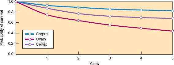
Figure 6.3 Relative Survival rates for invasive cancers of the cervix, corpus, and ovaries for women diagnosed in the United States in 2005. (Modified from Howlader N, Noone AM, Krapcho M, et al., eds. SEER Cancer Statistics Review, 1975–2010. Bethesda, MD: National Cancer Institute. Available at http://seer.cancer.gov/csr/1975_2010/. Based on November 2012 SEER data submission, posted to the SEER web site, 2013.)
Relative Survival
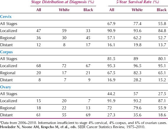
Relative survival is defined as the ratio of the observed survival rate for the patient group to the survival rate expected for a population with similar demographic characteristics. Relative survival rates for US women diagnosed in 2005 are shown in Figure 6.3 for the major gynecologic cancers and reveal that survival is best after cancer of the corpus, worst after cancer of the ovary, and intermediate after cancer of the cervix. Five-year relative survival rates are shown in Table 6.3 by type and stage of gynecologic cancer for US women. Stage at presentation and 5-year survival are most favorable for cancer of the corpus and least favorable for cancer of the ovary. In general, African Americans tend to be diagnosed at more advanced stages and have poorer survival compared with whites, especially for cancer of the cervix and corpus.
Table 6.3 Stage at Diagnosis for the Gynecologic Cancers and 5-Year Survival Rates for U.S. Womena
Etiologic Studies
In distinction to descriptive studies, etiologic studies examine the relationship between cancer occurrence and survival and personal factors such as diet and reproductive history. This relationship is often described by the epidemiologic parameters, relative risk, and attributable risk.
Relative Risk (RR) is the risk of disease or death in a population exposed to some factor of interest divided by the risk in those not exposed. Absence of association is indicated by an RR of 1 (null value); a number greater than 1 may indicate that exposure increases the risk of disease and a number less than 1 that exposure decreases the risk of disease.
Attributable risk is the risk of disease or death in a population exposed to some factor of interest minus the risk in those not exposed. The null value is 0; a number greater than 0 may indicate that exposure increases the risk of disease and a number less than 0 that exposure decreases the risk.
Case-control Study
In a case-control study, diseased and nondiseased populations are selected, and existing or past characteristics (exposures) are assessed to determine the possible relationship between exposure and disease. The investigator starts with diseased cases and nondiseased control subjects who are then studied to determine whether they had a particular exposure (before the illness). The odds that the cases were exposed (a/b) are compared with the odds that the control subjects were exposed (c/d) in a measure called the exposure odds ratio (Fig. 6.4).
Exposure Odds Ratio
The odds of exposure among cases divided by the odds of exposure among the control subjects is the exposure odds ratio; it approximates the RR. If an entire population could be characterized by its exposure and disease status, then the exposure odds ratio would be mathematically identical to the RR obtained in a cohort study. Because it is feasible to study only subsets of cases and control subjects, the exposure odds ratio in the sampled population approximates the RR, as long as the cases and control subjects actually sampled were not preferentially selected on the basis of their exposure status. Attributable risk cannot be directly calculated in a case-control study but is often estimated by a term called the etiologic fraction (4).
Cohort Studies
In a cohort study, the groups to be studied (the cohorts) are defined by characteristics (or exposures) that occur before the disease of interest, and the study groups are followed to observe the risk of disease in the cohorts. The investigator starts with exposed and nonexposed individuals who are monitored over time to identify the number of diseased cases that develop. The initial sizes of the cohort and the number of years cohort members are studied determine the person-time contributed by the cohorts.
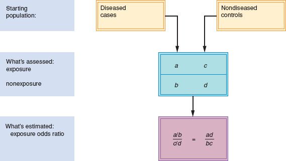
Figure 6.4 Case-control study design.
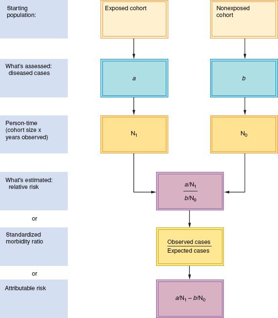
Figure 6.5 Cohort study design.
The investigator calculates the rates of disease in exposed and nonexposed subjects and determines the RR or attributable risk. For rare exposures, an investigator may use the general population as the unexposed group and calculate a parameter equivalent to the RR that is known as the standardized morbidity ratio (Fig. 6.5).
Standardized Morbidity or Mortality Ratio
The standardized morbidity or mortality ratio (SMR) is the observed number of exposed cohort members in whom disease developed, divided by the number expected if general population disease rates had prevailed in the cohort.
Cohort studies are further distinguished by when the exposure and outcome occurred or will occur in relation to when the investigator begins the study.
Retrospective Cohort Study
In a retrospective cohort study, the exposures and outcomes have already occurred when the study is begun. For example, studies of second cancers after therapeutic radiation are based on follow-up of women irradiated for cervical cancer 10 to 30 years ago. Medical records and death certificates are used to determine those who subsequently died of cancers other than cervical.
Prospective Cohort Study
In a prospective cohort study, the relevant exposure may or may not have occurred when the study began, but the outcome has not yet occurred. After the cohort is selected, the investigator must wait for the disease or outcome to appear in the cohort members. The Nurses’ Health Study is a good example of a prospective cohort study (5).
Clinical Trial
A clinical trial is a special type of prospective cohort study in which the investigator assigns a therapy or preventive agent in randomized fashion to minimize the possibility of bias accounting for different outcomes subsequently observed between treatment cohorts. Obviously, such studies cannot be used to assess a harmful effect of an exposure except as might occur as an unintended side effect of the therapy. Clinical trials are the only satisfactory way to assess the effect of different cancer therapies on disease recurrence or death because, in theory, they are able to overcome many of the biases that may affect case-control or cohort studies, as discussed in the next section.
Statistical Inference and Validity
Clinicians should understand issues affecting statistical significance and validity to evaluate studies claiming that some exposure causes cancer, a new therapy is superior to standard treatment, or a screening test can improve mortality.
Statistical Inference
Statistical inference is a process of drawing conclusions from data by hypothesis testing, during which a decision is made either to reject or not reject a null hypothesis. Hypothesis testing involves the following steps:
1. Observations are made and summarized by some statistical parameters, such as a mean, a proportion, or a relative risk.
2. A research question is stated in terms of a null hypothesis claiming no difference between the observed parameter and some theoretical value.
3. A statistical test is chosen based on the study design and nature of the parameters being studied.
4. The test statistic is calculated, and its associated p value is read from the appropriate statistical table or generated from a statistical program.
5. A p value less than the traditional 5% leads to the decision to reject the null hypothesis, whereas a value greater than 5% leads to the decision not to reject the null hypothesis. Errors are possible with either decision.
6. A confidence interval on the parameter may be constructed from the test results and defines the range in which the true value of the parameter is expected to fall. Precision refers to a characteristic of a parameter falling into a narrow confidence interval, a desirable feature of large studies.
Type I Error
The degree of conflict between the parameter observed and that assumed by the null hypothesis is summarized by the p value, alpha, or Type I error and indicates the probability of incorrectly rejecting the null hypothesis. In practice, an alpha level is chosen a priori, usually p = 0.05; and if the association tested has a p value less than the predetermined alpha level, then the results are considered statistically significant. It is important to note that when many tests are performed, some results will be observed by chance. One way to address this multiple testing issue, called Bonferroni correction, is to divide the alpha level by the number of tests being performed. If this method is used and 100 tests are performed, then the alpha level will be 0.05/100 or 0.0005.
Type II Error
A Type II or beta error indicates the probability of failing to reject the null hypothesis when, in reality, it is false. To calculate a beta error, an alternate hypothesis must be stated.
Power
Power is 1 minus the beta error and reflects the ability of a study to detect an actual effect. More precisely, power is the ability of a test statistic to detect differences of a specified size in test parameters. In planning a clinical trial, an investigator often calculates the power that a study will have to detect an association, given a certain study size and certain assumptions about the nature of the association. Small clinical trials that find no significant difference among therapies may be cited as evidence of “no effect of therapy” when the statistical power may have been well below the accepted target of 80% for a meaningful difference in response rates.
Statistical Distributions and Tests
There are no simple rules for determining which statistical test is appropriate in every situation. The choice depends on whether the variable is qualitative (nominal) or quantitative (numerical), what assumptions are made about the distribution of the parameter being measured, the nature of the study question, and the number of groups or variables being studied. For example, a chi-square test is used to test the null hypothesis that proportions are equal or that nominal variables are independent. The unpaired t-test is used to compare two means from independent samples, whereas the paired t-test compares the difference or change in a numerical variable for matched or paired groups or samples.
Validity
Validity has two components: internal validity and external validity. Internal validity means freedom from bias. Bias refers to a systematic error in the design, conduct, or analysis of a study that results in a mistaken conclusion and is commonly divided into observation bias, selection bias, and confounding. The external validity of a study refers to the ability to generalize the results observed in one study population to another. Although there is controversy about what characteristics of a study make for generalizability, it is clear that external validity is an issue only for those studies that possess internal validity, which is the main focus of this discussion.
Observation Bias
Observation bias or misclassification occurs when subjects are classified incorrectly with respect to exposure or disease. If misclassification was equally likely to occur whether the subject was a case or control or an exposed or nonexposed cohort member, then the observation bias would be nondifferential and would cause the RR to be biased toward the null value, 1. Alternatively, if misclassification was more likely to occur for case than control subjects or for exposed than nonexposed cohort members, then a falsely elevated (or decreased) RR might occur (e.g., if cases preferentially recalled or admitted to a particular exposure compared with control subjects).
Criteria for exposure or disease should be clearly defined to minimize observation bias and, whenever possible, exposure or disease confirmed from medical records. Ideally, researchers recording the disease status in a cohort study or exposure status in a case-control study should be unaware of the subject’s study group or blinded to key hypotheses. In a clinical trial, observation bias may be minimized by double blindness, when neither the subject nor the investigator knows which specific treatment the subject is receiving.
Selection Bias
Selection bias is an error that results from systematic differences in the characteristics of subjects who are and are not selected for study. For example, a selection bias might occur in a case-control study if exposed cases did much better or worse than nonexposed cases. If the case group consisted of long-term survivors, then they might have a different frequency of the exposure than newly diagnosed individuals. Selection bias may also occur in the process of selecting control subjects; for example, control subjects might be selected from hospitalized patients in a disease category that may, itself, relate to the exposure. Selection bias is less likely to occur in cohort studies or in population-based case-control studies, where most cases in a particular area are studied and control subjects are selected from the general population.
Confounding
Confounding occurs when some factor not considered in the design or analysis accounts for an association because that factor is correlated with both exposure and disease. Potential confounders for any cancer study are age, ethnicity, and socioeconomic status. Confounding may be controlled during the design of a study by matching cases to control subjects on key confounding variables, or during the analytic phase of the study by stratification or multivariate analysis. Stratifying means examining the association of interest within groups that are similar with respect to a potential confounder, whereas multivariate analysis is a statistical technique that controls for a number of confounders simultaneously.
In a clinical trial, confounding is avoided by randomization; that is, subjects are allocated to treatment groups by a chance mechanism such that prejudices of the investigator or preferences by the subject do not influence allocation of treatment. In practice, participant randomization assignments can be determined using computer-generated random numbers or random number tables found in most statistic textbooks (6,7). The initial table in the report of a clinical trial usually shows how the treatment groups compared with respect to age, ethnicity, or other important variables to demonstrate whether randomization indeed balanced key variables. Similar tables are helpful in case-control and cohort studies.
Other Criteria for Judging an Epidemiologic Study
Besides the important exercise of ruling out potential biases in a study, other criteria are invoked to decide whether an epidemiologic association is likely to be causal. The well-known British statistician Sir Austin Bradford Hill is credited with establishing the criteria that epidemiologists often use in judging whether an association is likely to be causal (8). Hill originally listed nine criteria, which have been restated over the years, but in one form or another, are considered when regulatory or legal issues arise in connection with an epidemiologic association. The following criteria are most important: Statistical significance, reverse causality, consistency, effect of removing the causal agent, bias and confounding, strength of the association, dose–response, and biologic credibility.
Statistical Significance of the Association
Applying the steps listed under statistical inference allows one to address the question of whether chance could have accounted for the observation. Mostly a p value cutoff of 5% is used to answer this question. A different bar is required in genome wide association studies (GWAS), in which risk predisposing variants are searched for using gene chips that can profile hundreds of thousands of genetic variants. Typically, genetic variations called single nucleotide polymorphisms (SNPs) are searched for and may number half a million or more. In such studies, p values on the order of 10−7 are common, and external validation is sought by retesting the associations identified in another or even several additional datasets.
Exposure Precedes the Disease
That exposure precedes disease in an obvious requirement. As discussed under “Observation Bias,” subjects are interviewed about exposures after their disease is diagnosed in a case-control study; therefore, cases may cite exposures that began because of symptoms or treatment of their illness resulting in “reverse causality.” Epidemiologists who conduct case-control studies generally censor exposures for some time period prior to disease diagnosis to minimize this limitation.
Consistency
Measurements that are in close agreement when repeated are said to be consistent. In the context of an epidemiologic association, RRs that are consistent among studies, especially those in which different study methods have been used, provide evidence for a causal association. However, the possibility that a systematic bias has affected all the studies should be considered. Consistency can be assessed in a formal manner by performing a study called a meta-analysis.
In a meta-analysis, results from independent studies examining the same exposure (or treatment) and outcome are combined, so that a more powerful test of the null hypothesis may be conducted. As part of the meta-analysis, a test for heterogeneity is performed to indicate whether there have been any statistical differences among the results of different studies. The meta-analysis has become an important component of evidence-based medical reviews. For example, oral contraceptive use was less common in ovarian cancer cases compared to controls in 45 studies; when the results of all studies were combined in a meta-analysis, women who had ever used oral contraceptives had an estimated 17% reduction in ovarian cancer risk compared to women who had never used oral contraceptives (9).
Removal of the Agent Results in a Reduction of Disease Frequency
In diseases caused by infection, showing that treatment of the infection or protection by vaccination cured or prevented the disease would satisfy this criterion, and has been clearly demonstrated for HPV vaccination and high-grade CIN. In chronic disease epidemiology, this criterion might be addressed by showing a correlation between calendar year and disease occurrence for an exposure that was relatively limited in time or has changed over time. The increased incidence of endometrial cancer that followed the expanded use of estrogen therapy for the menopause and the decline that followed the addition of a progestogen satisfy this criterion. The decline in breast cancer occurrence following the Women’s Health initiative study showing an increased incidence of the disease in women using combined hormone replacement therapy (HRT), and the subsequent decreased use of HRT, would be another example.
Strength of the Association
It is common to hear clinical epidemiologists argue that an RR or OR of 2 is a benchmark as the minimum for associations likely to be causal (10). Bradford-Hill himself said: “We must not be too ready to dismiss a cause-and-effect hypothesis merely on the grounds that the observed association appears to be slight. There are many occasions in medicine where this is in truth so.” He cited the case of coronary thrombosis and smoking.
The argument that risks less than 2 cannot be causal should be rigorously challenged. An overall summary risk less than 2 does not rule out a stronger association for certain histologic types of gynecologic cancer, certain categories of exposure, or for women with certain characteristics. The question of whether an association less than 2 can be causal is addressed by recent genome-wide association studies (GWAS), which test hundreds of thousands of genetic variants called SNPs in cases and controls. GWAS studies have revealed genetic polymorphic variants that individuals are born with that may increase the risk for various cancers, including ovarian cancer. Thus, SNPs rs8170 and rs2363956 on chromosome 19 are associated with ORs of 1.16 and 1.18 for serous ovarian cancer, respectively. These associations are almost certain to be real, based on three phases of evaluation in over 5,900 cases and 13,000 controls, and p values of 10−9 and 10−11, respectively (11).
Dose–Response
A dose–response (or biologic gradient) refers to a consistent increase (or decrease in the case of a protective exposure) in risk, corresponding to increasing levels of the exposure. Whether there is an association is addressed by a simple “yes” or “no” answer to a question about exposure. Individuals who answer “yes” and had a particular exposure should be asked additional questions about the frequency and duration of the exposure. To categorize dose–response as precisely as possible, it is necessary to combine both frequency and duration, similar to that which is done for smoking when a “pack-years” variable is calculated (i.e., the number of packs per day smoked multiplied by the number of years smoked). A key issue in calculating dose–response is whether those who have never had the exposure should be included in the calculation, or whether the dose–response should be calculated only for those who have had the exposure.
Biologic Credibility
Biologic credibility requires that we ask whether the association makes biologic sense in terms of what is known about the biology of the cancer or the exposure, and whether animal or cell line experiments support an association. Any epidemiologic study claiming a new association needs to address the biologic credibility of the association. Bradford-Hill cautioned against making this an essential criterion: “It will be helpful if the causation we suspect is biologically plausible. But this is a feature I am convinced we cannot demand. What is biologically plausible depends upon the biologic knowledge of the day” (8).
Cancer Risk and Prevention
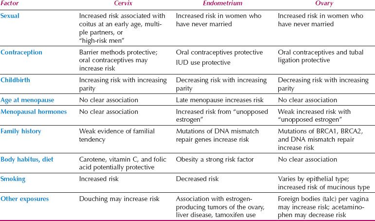
Risk factors for the gynecologic cancers are presented, along with the application of this information to cancer prevention. Table 6.4 summarizes major epidemiologic risk factors for cervical, endometrial, and ovarian cancer.
Cervical Cancer
Invasive squamous cell carcinoma of the cervix is the end stage of a process beginning with atypical transformation of cervical epithelium at the squamocolumnar junction, leading to CIN of advancing grades, and eventually invasive disease. Risk factors for cervical cancer are those associated with atypical transformation and those that influence persistence and progression of disease.
Factors associated with atypical transformation largely relate to sexual practices that increase the opportunity for human papilloma virus (HPV) infection. Early age at first intercourse may be important, because adolescence is a period of heightened squamous metaplasia, and intercourse at this time may increase the likelihood of atypical transformation (12). The woman who has intercourse with multiple partners, or with a “high-risk” male who has had contact with multiple partners, increases the likelihood of her exposure to HPV and cervical cancer (13–15). An estimated 27% of US women aged 14 to 59 have a prevalent HPV infection, and the rate is 45% among women aged 20 to 24 years (16). Over a lifetime, an estimated 79% of women will be infected with HPV at least once (17). The link with HPV infection means that a woman can decrease her risk of cervical cancer by vaccination, safe sexual practices, and use of barrier methods of contraception (18). In addition, both observational studies and randomized trials suggest that male circumcision decreases the risk of HPV infection and cervical cancer in their partners (19–21).
Table 6.4 Risk Factors for Gynecologic Cancers
Stay updated, free articles. Join our Telegram channel

Full access? Get Clinical Tree


