Statistical innovations in cancer research
J. Jack Lee, PhD, MS, DDS  Donald A. Berry, PhD
Overview
Cancer research is rapidly changing, with fast-growing numbers of possible cancer targets and cancer drugs to investigate and no end in sight. Advances in genomics, proteomics, and epigenetics provide remarkably detailed profiles of each patient’s tumor and, as a result, allow science to consider each patient as unique, with the goal of delivering precision medicine to each patient. The low success rates of late-phase clinical oncology trials and high costs of bringing new drugs to market, however, have necessitated changes in the drug-development process. Statistical innovations can help in the design and conduct of clinical trials to facilitate the discovery and validation of biomarkers and streamline the clinical trial process. The application of Bayesian statistics provides a sound theoretical foundation that can encourage the development of adaptive designs to improve trial flexibility and efficiency while maintaining desirable statistical-operating characteristics.
The principal goals of the innovations presented in this chapter are to (1) use information from clinical trials more efficiently in drawing conclusions about treatment effects, (2) use patient resources more efficiently while treating patients who participate in clinical trials as effectively as possible, and (3) identify better drugs and therapeutic strategies more rapidly, moving them more quickly through the development process. The underlying premise is to exploit all available evidence, placing information gleaned from an ongoing clinical trial into the context of what is already known. The innovations considered are intuitively appealing. However, some are controversial. Some are being used in actual clinical trials while others are still being developed and evaluated for such use.
This chapter addresses two types of innovations. One is a natural extension of the traditional practice of frequentist statistics. The other type is based on a Bayesian statistical philosophy. The Bayesian approach is tailored to real-time learning (as data accrue), and the frequentist approach is tied to particular experiments and to the experiment’s design. However, there is substantial overlap between these complementary approaches.
The main topics covered in this chapter include the following. The introduction of basic probability theory and Bayesian approach is explained through examples. Differences between frequentist and Bayesian methods are compared and contrasted. The development of adaptive designs by applying outcome adaptive randomization, predictive probability, interim and extraim analyses, and factorial design is discussed. In addition, hierarchical modeling can be utilized to synthesize information available from the trial as well as external to the trial. Seamless phase I/II and II/III designs can be applied to shorten the drug-development period. Platform designs can be constructed to evaluate many drugs simultaneously. The application of these statistical innovations is illustrated in the BATTLE trials and I-SPY 2 trial. Finally, information on computing resources for the design and implementation of innovative trials is given.
Cancer research (and medical research, in general) is rapidly changing; the number of possible cancer targets and cancer drugs to investigate is growing, with no end in sight. Advances in genomics, proteomics, and epigenetics provide remarkably detailed profiles for each patient’s tumor and, as a result, allow science to consider each patient as unique. Modern computing has supported these advances, allowing statisticians to simulate trials with complicated designs and to evaluate design properties such as statistical power and false-positive rate. The basic requirement is that the design be specified prospectively.
The low success rates of late-phase clinical oncology trials1–3 and high costs of bringing new drugs to market4 have necessitated changes in the drug-development process. Recognizing the need to modernize, the FDA issued its Critical Path Opportunities Report in March 2006, identifying biomarker development and streamlining clinical trials as essential changes to be made in this process.5 Further guidance was then issued by centers within the FDA: The Center for Devices and Radiological Health (CDRH) published initial guidelines for using Bayesian statistics in medical device clinical trials in 2006 and final guidelines in 2010.6 The Center for Biologics Evaluation and Research (CBER) and the Center for Drug Evaluation and Research (CDER) issued a joint guidance document for planning and implementing adaptive designs in clinical trials.7 In addition, CDRH released a draft guidance on adaptive designs for medical device clinical studies in 2015.8
The principal goals of the innovations presented in this chapter are to (1) use information from clinical trials more efficiently in drawing conclusions about treatment effects, (2) use patient resources more efficiently while treating patients who participate in clinical trials as effectively as possible, and (3) identify better drugs and therapeutic strategies more rapidly, moving them more quickly through the development process. The underlying premise is to exploit all available evidence, placing information gleaned from an ongoing clinical trial into the context of what is already known. The innovations considered are intuitively appealing. However, some are controversial. Some are being used in actual clinical trials while others are still being developed and evaluated for such use.
This chapter addresses two types of innovations. One is a natural extension of the traditional practice of frequentist statistics. The other type is based on a Bayesian statistical philosophy. Readers who are familiar with Bayesian ideas may wish to skip some Bayesian sections. The Bayesian approach is tailored to real-time learning (as data accrue), and the frequentist approach is tied to particular experiments and to the experiment’s design. However, there is substantial overlap between these complementary approaches. Much of this chapter’s development of clinical trial design employs the Bayesian approach as a tool for finding designs that tend to treat patients in the clinical trial more effectively and that identify better drugs more rapidly. However, the frequentist properties (such as false-positive rate and power) of the design thus derived can always be found, often requiring simulation. Ensuring that a design has prespecified frequentist properties means that the Bayesian approach can be used to design trials with good frequentist properties.
Preliminaries
The basis of all experimentation is comparison. Evaluating an experimental therapy in a clinical trial requires information about the outcomes of the patients had they received some other therapy. The best way to address this issue is to randomize patients to the experimental therapy and to some comparison therapy. Although there are ways to learn without randomizing, there are limitations to approaches that do not employ randomization. Moreover, randomization does not require equal assignment probabilities to the therapeutic strategies, or “arms,” being compared. Unbalanced randomization is possible, either with fixed ratios or adaptive ratios, that is, such that assignment probabilities depend on data accumulating in the trial. (The latter possibility is the principal focus of this chapter.)
Most clinical trials are conducted in accord with a protocol, which aims to evaluate the treatment effect as a whole.9 Protocols may refer to retrospective or sporadic collection of data, but they are usually prospective. Clinical trials are always prospective. A prospective protocol describes how the trial is to be conducted, including how patients will be assigned to a therapy and when the trial will end. Deviations from a protocol may make scientific inferences from the trial difficult or impossible (although they may be necessary at times to avoid exposing participants to unnecessary risks). Valid inference can only be made based on sound statistical theory in properly conducted trials.
Bayesian approach
This section shows how Bayesian learning takes place and how the Bayesian approach relates to the more traditional frequentist approach. It is necessarily superficial. Further reading includes a comprehensive but elementary introduction to Bayesian ideas and methods,10 discussions of their role in medical research,11 and of clinical trials in particular,12–15 and books describing more advanced Bayesian methods.16, 17
Bayesian updating
The defining characteristic of any statistical approach is how it deals with uncertainty. In the Bayesian approach, uncertainty is measured by probability. Any event whose occurrence is unknown has a probability. The frequentist approach uses probabilities as well, but in a more restricted manner, as described hereafter. Examples of probabilities in the Bayesian approach that do not have frequentist counterparts include the following: The probability that the drug is effective, the probability that patient Smith will respond to a particular chemotherapy, and the probability that the future results in the trial will show a statistically significant benefit for a particular therapy.
The Bayesian paradigm is one of learning. As information becomes available, one updates one’s knowledge about the unknown aspects of the process that is producing the information. The fundamental tool for learning under uncertainty is Bayes’ rule. Bayes’ rule relates inverse probabilities. An example that will be familiar to many readers is finding the positive predictive value (PPV) of a diagnostic test: In view of a positive test result, what is the probability that the individual being tested has the disease in question? It can be considered as the “inverse probability” of a positive test given the presence of the disease, which is called the test’s sensitivity. PPV also depends on the test’s specificity, which is the probability of a negative test, given that the individual does not have the disease. Moreover, PPV depends on the prevalence of the disease in the population. In applying Bayes’ rule to statistical inference, the analog of PPV is the “posterior probability” that a hypothesis is true, given the experimental results. The analog of disease prevalence is the “prior probability” that the hypothesis is true.
Consider an overly simplified numerical example, one with only two possible response rates (r): r = 0.75 and r = 0.50. If you are accustomed to thinking about PPV for diagnostic tests, consider one of these to be that the “patient has the disease” and the other to be that the “patient does not have the disease.” The question is this: Is r equal to 0.75 or 0.50? Before any experimentation, these two possibilities are regarded to be equally likely: P(r = 0.75) = P(r = 0.50) = 1/2.
The focus of the Bayesian approach is learning. Probabilities are calculated as new information becomes available, and is taken to be “given.” Statisticians have a notation that facilitates thinking about and calculating probabilities as new information accrues. They use vertical bars to separate the unknown event of interest from known quantities (or taken to be given): P(A|B) is read “probability of A given B.” Assign R for tumor response and N for nonresponse. Using this notation, for example, P(R|r = 0.75) = 0.75. More interesting is the probability of r = 0.75, given a tumor response: P(r = 0.75|R). These two expressions are reciprocally inverse, with the roles of the event of interest and the event being assumed. Bayes’ rule connects the relationship between these two expressions, namely that the updated (posterior) probability of r = 0.75 is as follows:

The denominator on the right-hand side of the equation follows from the law of total probability:
That is, P(R) is the average of the two response rates under consideration, 0.75 and 0.50, where the average is with respect to the corresponding prior probabilities—half each in this example. Substituting the numerical values into Bayes’ rule, the posterior probability of r = 0.75 is as follows:

Therefore, the new evidence boosts the probability of r = 0.75 from 1/2 (or 50%) to 60%. As the total probability is 100%, the evidence in a single response lowers the probability of r = 0.50 from 50% to 40%.
Consider a second independent observation. The probability of r before this second observation is the posterior probability of the first observation. If the second observation is also a response, then a second application of Bayes’ rule applies to give P(r = 0.75|R, R) = 9/13 = 69%, which is a further increase from the previous values of 50% and 60%. On one hand, if the second observation is a nonresponse, then P(r = 0.75|R, N) = 3/7 = 43%, a decrease from 60%. This process can go on indefinitely, updating either after each observation or all at once on the basis of whatever evidence is available. The current probabilities of the various possible values of response rate r can be found at any time. These probabilities depend on the original prior probability and on the intervening observed data. This process of updating and real-time learning is an important advantage of the Bayesian approach to designing and conducting clinical trials.
The example mentioned previously considered only two possible values of r. More realistically, the response rate r may be any number between 0 and 1. The left-hand panel in Figure 1a shows a constant or flat curve that is a candidate for prior distribution. The flat curve indicates that the probability is spread equally over this range of values of r. This might be termed an “open-minded prior distribution” because the posterior distribution depends almost entirely on the evidence from the experiment at hand. After a single-tumor response, Bayesian updating serves to change the probability distribution to the one shown in the right-hand panel of Figure 1a—that is, the right-hand panel is the posterior distribution after observing R when the prior distribution is the one shown in the left-hand panel. The shift in the distribution to larger values of r corresponds to the intuitive notion that larger response rates become more likely after observing R. Bayes’ rule quantifies this intuition.
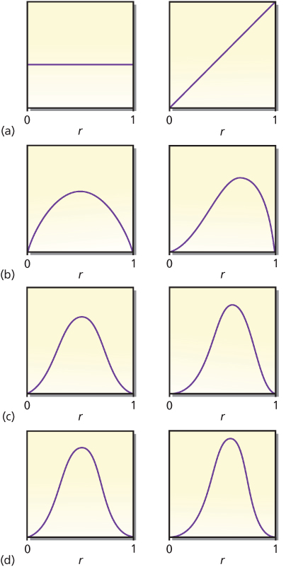
Figure 1 Prior distributions of response rate r. The left-hand panel in each pair is the prior distribution of response rate r. The right-hand panel is the posterior distribution of r after having observed a response in a single patient. The (predictive) probability of a response for each left-hand panel is 0.500, increasing in the right-hand panels to 0.667, 0.600, 0.571, and 0.556 in cases (a), (b), (c), and (d), respectively. Changes are greater and learning is more rapid when the prior distribution reflects greater uncertainty.
There are many candidate prior distributions other than the first one shown in Figure 1a. Three other prior/posterior pairs are shown in Figure 1b–d. The right-hand panel within each pair is the posterior distribution after observing R when the prior distribution is the one shown in the left-hand panel. Moreover, the left-hand curves in Figure 1b–d are themselves posterior distributions for the right-hand curves in Figure 1a–c, respectively, but in the situation when the observation is an N. Intuitively, after a nonresponse, the concentration of probabilities shifts to smaller values of r. Mathematically, observing R means to multiply the current distribution by r (the response rate) and renormalize it so that the area under the curve is 1. Similarly, observing an N means to multiply by (1 − r), the rate of nonresponse.
An implication is that moving left to right and top to bottom in Figure 1 corresponds to starting with the prior distribution in the left-hand panel of Figure 1a and observing RNRNRNR. The eight curves shown in Figure 1 are proportional to the following respective functional forms: 1, r, r(1 − r), r2(1 − r), r2(1 − r)2, r3(1 − r)2, r3(1 − r)3, and r4(1 − r)3. Each observation of response increases the exponent of r by 1, and each observed N increases the exponent of (1 − r) by 1. As is evident in the figure, additional observations lead to narrower distributions. As the number of observations increases, the distribution tends to concentrate about a single point, which is the “true” value of r, the response rate that produces the observations. Free software that provides a visual demonstration of the Bayesian update in the context of the so-called beta-binomial distribution can be downloaded at https://biostatistics.mdanderson.org/SoftwareDownload/SingleSoftware.aspx?Software_Id=96.
The principal message of this section is not the numerical calculation defining the updated distribution, but the fact that updated distributions can be found using the Bayesian approach at any time during a clinical trial.
Prior probabilities
Bayesian updating requires a starting point: a prior distribution of the various parameters. In the example, one must have a probability distribution for response rate r in advance of or separate from the experiment in question. This prior distribution may be subjectively assessed or based explicitly on the results of previous experiments. In some settings, such as some regulatory scenarios, an appropriate default distribution is noninformative or open-minded10, 13 in the sense that all possible values of the parameters are assigned the same prior probabilities. The left-hand panel of Figure 1a is an example.
Noninformative or flat prior distributions limit the benefits of taking a Bayesian approach when they ignore information that is available from outside the experiment. However, the benefit of employing Bayesian updating may be substantial even if one starts with a flat distribution that does not reflect anyone’s assessment of the prior information. Flat prior distributions serve some important roles. One is that it may be helpful to distinguish the evidence in the data in the experiment under consideration from that present before the experiment. Another is that the Bayesian conclusions that arise from using flat prior distributions are often the same as the corresponding frequentist conclusions.
Prior distributions are usually based on historical data. Suppose that a similar drug (or the same drug in a possibly different patient population) gave a response rate of 50% in 20 patients: 10 responders and 10 nonresponders. The corresponding likelihood of response rate r (see the section titled “Frequentist/Bayesian Comparison”) is r10(1 − r)10. Given that there may be differences between the historical setting and that of the current trial, it would not be reasonable to use this information directly without any modification as a prior distribution for r, but it would be appropriate to somehow exploit this relevant information. One possibility (another is described in the section titled “Hazards over Time”) is to discount the historical evidence as it applies to the context of the current trial. For example, weighing an historical observation as having the information equivalent of 30% of that of a current observation would mean using a prior distribution proportional to r3(1 − r)3. This is the distribution shown in Figure 1d, left-hand panel.
Robustness
In the presence of enough data, essentially all observers will have similar posterior distributions; this is robustness. An implication is that the particular prior distribution assumed does not matter much when the sample size is moderate or large. As an example, consider the eight distributions shown in Figure 1 and think of each of them in turn as being the prior distribution of a different person. Parameter r is the response rate to a particular drug. Suppose that 40 patients are treated in a trial and 20 of them respond. Applying the principle of robustness, the eight people in question will come to very nearly the same conclusion about the drug’s response rate. The eight posterior distributions are shown in Figure 2. The curves are nearly superposed. The eight 95% probability intervals will also be very similar. The data outweigh any of the prior distributions shown in Figure 1.
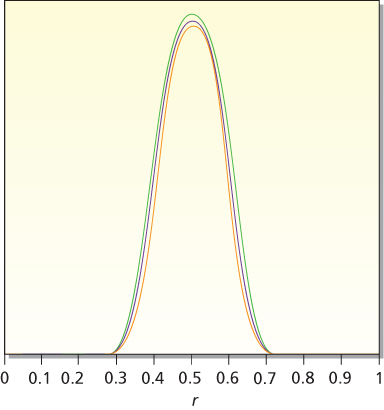
Figure 2 Posterior distributions for response rate r based on an experiment with 20 responses and 20 failures. The eight prior distributions considered are the eight distributions shown in Figure 1. Except for proportionality constants, these are 1, r, r(1 − r), r2(1 − r), r2(1 − r)2, r3(1 − r)2, r3(1 − r)3, and r4(1 − r)3. The corresponding posterior distributions are proportional to r20(1 − r)20, r21(1 − r)20, r21(1 − r)21, r22(1 − r)21, r22(1 − r)22, r23(1 − r)22, r23(1 − r)23, and r24(1 − r)23. These eight posterior distributions are very similar, demonstrating the robustness principle.
If two prior distributions are markedly different and the corresponding information contained in the prior distribution is strong, then robustness still applies, but it could take a good deal of data to bring two disparate distributions close together.
Frequentist/Bayesian comparison
In the frequentist approach, hypotheses and parameters do not have probabilities. Rather, probability assignments apply only to data, with particular values assumed for given unknown parameters in calculating these probabilities. For example, the ubiquitous p-value is the probability of data as or more extreme than the observed data assuming that the null hypothesis is true. In symbols:
- Frequentist p-value: P(observed or more extreme data |H0)
- Bayesian posterior probability: P(H0| observed data)
It is easy to confuse these two concepts. A p-value is commonly interpreted as the probability of no effect, and 1 minus the p-value as the probability of an effect. This interpretation is wrong. This is trying to have a Bayesian posterior probability without a prior probability, which is impossible.
There are two important differences between a frequentist p-value and a Bayesian posterior probability. One is the inversion of the conditions: what is assumed in the former has a probability in the latter. The second difference is that p-values include probabilities of results other than those observed in the experiment.
As an example, consider a single-arm phase II trial for testing H0: r = 0.5 versus H1: r = 0.75. Assuming a type I error rate α = 5%, a sample size of n = 33 gives 90% power. Suppose that the final results are of 22 responses of 33 patients, the (frequentist) one-sided p-value is the probability of 22 or more responses of the 33 patients, assuming the null hypothesis, H0: r = 0.5. Under this assumption, the probability of observing 22, 23, 24, … responses is 0.0225 + 0.0108 + 0.0045+ … = 0.0401. As this p-value is less than 5%, observing 22 responses is said to be “statistically significant.”
The Bayesian measure is the posterior probability of the hypothesis that r = 0.75 (which is 1 − the probability of r = 0.5) given 22 responses out of 33. (As indicated earlier, the Bayesian calculation depends only on the probability of the data actually observed, 22 responses of 33, while the frequentist calculation also includes probabilities of 23, 24, etc., responses.) Using Bayes’ rule:

As mentioned in the equation, the denominator follows from the law of total probability assuming H0 and H1 being equally likely before observing the data:
Therefore,
The calculation considers just two hypotheses, r = 0.5 and r = 0.75. In considering other values of r, Bayes’ rule weighs them by P(22 of 33|r), which is called the likelihood function of r. The likelihood function is pictured in Figure 3. It indicates the degree of support for response rate r provided by the observed data. Values of r having the same likelihood are equally supported by the data. Only relative likelihoods matter. For example, conclusions about r = 0.5 versus 0.75 depend only on the ratio of their likelihoods, 0.0823 and 0.0225, values that are highlighted in Figure 3. Because 0.0823/0.0225 = 3.66, the data lend 3.66 times as much support to r = 0.75 as they do to r = 0.5.
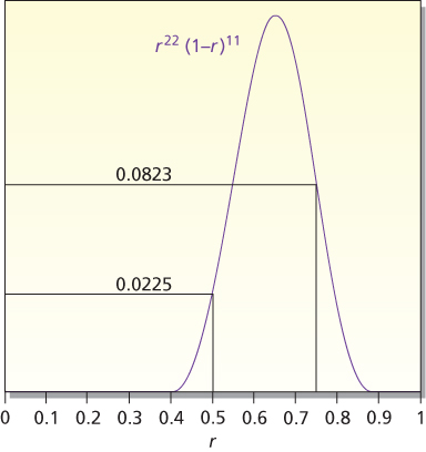
Figure 3 Likelihood of r for 22 responses out of 33 observations. The likelihood is P(22 of 33|r), which is proportional to r22(1 − r)11. The likelihoods at r = 0.5 and 0.75 are highlighted. These values are used in the calculational example in the text.
The conclusions of the two approaches are different conceptually and numerically. In the frequentist approach, the results are statistically significant, with p-value = 0.0401. Some researchers interpret statistical significance to mean that H0 is unlikely to be true. That is not what it means. It means that the observed data are unlikely when H0 is true. The Bayesian posterior probability of H0 directly addresses the question of the probability that H0 is true. This probability is 0.215. Although smaller than the prior probability of 0.50 (because the data point somewhat more strongly to H1 than to H0), it is five times as large as the p-value!
Interval estimates also have different interpretations in the two approaches. In the Bayesian approach, one can find the probability that a parameter lies in any given interval. In the frequentist approach, confidence intervals have a long-run frequency interpretation for fixed and given parameters. So it is not correct to say that a 95% confidence interval has a probability of 95% containing the parameter of interest. Despite the different interpretations, there is a point of agreement between the two approaches. In other words, if the prior distribution is flat (e.g., the left-hand panel of Figure 1a), then the Bayesian posterior probability of a confidence interval is essentially the same as the frequentist level of confidence. For example, if the prior distribution is flat, then the Bayesian posterior probability, indicating that a parameter lies in its 95% confidence interval, is in fact 95%. For prior distributions that are not flat, the posterior probability of a 95% confidence interval may be greater than or less than 95%. If the historical data upon which the prior distribution is based are consistent with those from the current experiment, then the posterior probability indicating that the parameter is in the 95% confidence interval will be >95%. If the historical data are different from those in the current experiment, then the probability that the 95% confidence interval contains the true parameter will typically be <95%.
Predictive probabilities
The ability to predict the future—with the requisite uncertainty—is important for designing and monitoring trials. The Bayesian approach allows for calculating probabilities of future results without having to assume that any particular hypothesis is true. The process is straightforward, at least logically if not mathematically. For a specified experimental design, one finds the conditional probabilities of the future data for each parameter value and averages them with respect to the current probabilities of the various parameter values. Predictive probabilities are exploited extensively in this chapter.
Consider the 33-patient trial described earlier. Suppose that the first 16 patients have been treated, with 13 responses and 3 nonresponses. What will be the results after the full complement of 33 patients is available? The number of responses will be between 13 and 30, but not all events are equally likely. In particular, it seems most unlikely that there will be no responses in the next 17 patients after having seen 13 of the first 16 patients, and it is.
It might seem reasonable to use an estimate of r (e.g., the current rate, 13/16 = 0.81) and calculate the probabilities of the results of the next 17 patients, assuming this value of r, but this could be wrong. Such a calculation incorporates the uncertainty in the future data for the given r, but fails to incorporate uncertainty in r. Bayesian predictive probabilities incorporate both types of uncertainty. Table 1 shows the results, assuming just two values of r, 0.5 and 0.75. The first column (the leftmost column) lists the possible numbers (S) of responses after 33 patients. The second and third columns show the probabilities of the possible values of S for these two values of r. The corresponding probabilities without conditioning on r are shown in the fourth column. This is a weighted average of the second and third columns. The weights are the respective probabilities of the two values of r conditional on having observed 13 responses in the first 16 patients: 0.039 for r = 0.5 and 0.961 for r = 0.75. The fourth column evinces greater variability (greater standard deviation) than either of the previous two columns. Typically, when all values of r between 0 and 1 are considered (i.e., all values have positive probability), predictive probabilities reflect greater uncertainty about future results than when conditioning on a particular value of r. (The rightmost column of Table 1 is discussed in the next section.)
Table 1 Predictive probabilities of number S of responses after 33 patients, given 13 responses in the first 16 patients
| S(of 33) | P(S|r = 0.5) | P(S|r = 0.75) | P(S) | P(Hl) |
| 13 | 0.0000 | 0.0000 | 0.0000 | 0.0002 |
| 14 | 0.0001 | 0.0000 | 0.0000 | 0.0006 |
| 15 | 0.0010 | 0.0000 | 0.0000 | 0.0017 |
| 16 | 0.0052 | 0.0000 | 0.0002 | 0.0050 |
| 17 | 0.0182 | 0.0000 | 0.0007 | 0.0148 |
| 18 | 0.0472 | 0.0001 | 0.0019 | 0.0432 |
| 19 | 0.0944 | 0.0005 | 0.0042 | 0.1192 |
| 20 | 0.1484 | 0.0025 | 0.0082 | 0.2887 |
| 21 | 0.1855 | 0.0093 | 0.0162 | 0.5491 |
| 22 | 0.1855 | 0.0279 | 0.0341 | 0.7851 |
| 23 | 0.1484 | 0.0668 | 0.0701 | 0.9164 |
| 24 | 0.0944 | 0.1276 | 0.1263 | 0.9705 |
| 25 | 0.0472 | 0.1914 | 0.1857 | 0.9900 |
| 26 | 0.0181 | 0.2209 | 0.2129 | 0.9966 |
| 27 | 0.0052 | 0.1893 | 0.1820 | 0.9989 |
| 28 | 0.0010 | 0.1136 | 0.1091 | 0.9996 |
| 29 | 0.0001 | 0.0426 | 0.0409 | 0.9999 |
| 30 | 0.0000 | 0.0075 | 0.0072 | 1.0000 |
Note: Columns P(S|r = 0.5) and P(S|r = 0.75) assume the indicated value of r in calculating the probability. Column P(S) is the weighted average of the two previous columns, where the respective weights are 0.039 and 0.961. The last column gives P(Hl), the probability of HI (r = 0.75), given S responses after 33 patients.
For convenience in this example, equal prior probabilities are assumed: P(H1) = P(H0) = 0.5. Although there is no vertical bar “|” in these expressions, these probabilities can depend on other available evidence, such as results of earlier clinical and preclinical trials. There may be additional information from biological assessments, such as when considering targeted therapies. These overall conditions are taken to be understood in setting down P(H0) and P(H1).
Bayesian versus frequentist interim analyses
There are numerous commonalties and a few differences between the Bayesian and frequentist approaches. This section addresses a principal difference. In the Bayesian approach, one makes an observation and updates the probabilities of the various hypotheses. This simple process implies a degree of flexibility that is difficult to mimic in the frequentist approach.
Consider the trial design described previously, with n = 33 patients and testing H0: r = 0.5 versus H1: r = 0.75. Observing 22 or more responses will be sufficient to reject H0 in favor of H1 (with a one-sided 5% type I error rate). However, assigning 33 patients to an experimental therapy without assessing interim results is ethically problematic and would likely be questioned by institutional review boards. If the results are conclusive (either positive, strongly suggesting r > 0.5, or negative, suggesting r ≤ 0.5) part of the way through the trial, then the trial should be stopped. Suppose that after 16 patients, one finds that 13 respond and 3 do not, from a Bayesian perspective, the updated probability of H1 is 96.1% (assuming prior probability P(H0) = 0.5).
Whether this probability is “conclusive” is not clear. The decision as to whether to continue a trial is complicated. It depends on the consequences of the trial, given the current results and also given the future results. In the Bayesian approach, the consequences of future results can be weighed by their predictive probabilities; for example, suppose that the impact of the trial depends on whether the posterior probability of H1 is > 95% when the data from the full complement of 33 patients become available, then one can calculate the predictive probability of this event. The rightmost column in Table 1 shows the posterior probability of H1 assuming S responses of 33 patients. To achieve >95% posterior probability requires at least 24 responses in the 33 patients. The probability of this event is the sum of the probabilities for S ≥ 24 (the fourth column in Table 1), which is 0.8642. Although the current probability of H1 is > 95%, owing to the uncertainty in S and in r, this characteristic will be lost with probability 1 − 0.8642 = 0.1358. That this has moderate probability indicates the tentative nature of the current conclusion. The possibility that the current conclusion is moderately likely to change can be factored into the decision to continue the trial.
If the predictive probability that the current conclusion will be maintained is sufficiently high, then one may reasonably decide to stop a trial. This is true for both claims of futility and superiority. The possibility of stopping a trial early on the basis of predictive probability should be stated explicitly in the trial’s protocol.
The focus of the frequentist perspective is the type I error rate, α. This is the probability of rejecting H0 when H0 is true, which depends on the trial design. For a fixed sample size of 33 patients, the calculation is straightforward. Rejecting H0 for ≥22 responses means α = 0.0401 (see the previous section). The calculation becomes more complicated when there is a possibility of stopping the trial early. In the example, if the trial is stopped and H0 is rejected, when there are 12 or more responses in the first 16 patients, then α is increased because there is additional opportunity for rejecting H0. Assuming r = 0.5, the probability of rejecting H0 is now 0.0640. Because this is greater than 0.05, the convention is to modify the stopping and rejection criteria to reduce α to about 0.05. For example, rejecting only if there are 13 responses or more out of 16 patients treated, or if there are 22 or more responses after 33 patients are treated, gives an overall type I error rate of 0.0450.
It follows that it is more difficult to draw a conclusion of statistical significance when there are interim analyses. The reason is that the type I error rates are calculated assuming that a particular hypothesis (the null hypothesis of no effect) is true. In a sense, an investigator is penalized for interim analyses in the frequentist approach. There are no such penalties for interim analyses in a Bayesian perspective. The reason is that Bayesian probabilities are not conditional on the basis of any particular hypothesis.
Although it is not a Bayesian quantity, the type I error rate of any Bayesian design, however complicated, can be evaluated. If the design has interim analyses, then such a calculation incorporates appropriate penalties. This calculation is straightforward in a simple example such as that given earlier. In more complicated settings, it can require Monte Carlo simulations.
A breast cancer trial illustrates some advantages of a Bayesian design.18 Women with breast cancer who were at least 65 years of age were randomized to receive either standard chemotherapy or capecitabine. The sample size was expected to be 600–1800. After the 600th patient had enrolled in the trial, and following the protocol, predictive probabilities were calculated. Calculations were made of the predictive probability of statistical significance given the present sample size and with additional patient follow-up at the present sample size. If that achieved a predetermined level, patient accrual would stop, but observations of the existing patients would continue. The predictive probability cutoff point was achieved at the first interim analysis and so accrual stopped (the final sample size was 633). Indeed, the study later showed that the women in this study population who were treated with standard chemotherapy had a lower risk of breast cancer recurrence and death than women treated with capecitabine.19
Analysis issues
The purpose of this section is to consider two types of analytical issues. The first is an extension of the previous section. The second is unrelated to the first and deals with a particular aspect of survival analysis.
Hierarchical modeling: synthesizing information
When analyzing data from a clinical trial, other information is usually available about the treatment under consideration. This section deals with a method called hierarchical modeling. One of its uses is synthesizing information from different sources. The method applies in many settings, including meta-analysis and incorporating historical information. A hierarchical model is a random-effects model. In a meta-analysis, one level of the experimental unit is the patient (within a trial) and the second level is the trial itself. Hierarchical models also apply for design issues such as combining results across diseases or disease subtypes and for such seemingly disparate issues such as cluster randomization. Design issues for hierarchical modeling are considered in the next section.
Consider a phase II trial in which 21 of 33 patients responded. The one-sided p-value is 0.08 for the null hypothesis H0: r = 0.50, and so the results are not statistically significant at the 5% level. Now consider an earlier phase I trial using the same treatment in which 15 of 20 patients responded. This information seems relevant, even if the population being treated might have been somewhat different and the trial might have been conducted at a different institution. However, it is not obvious how to incorporate the information into an analysis. The frequentist approach is experiment specific, which requires imagining that the two trials are part of some larger experiment. If one assumes that the entire set of data resulted from a single trial involving 53 patients with 36 responses, then from a frequentist perspective this would lead to a p-value of 0.0063, which is highly statistically significant. However, this conclusion is wrong because the assumption is wrong. Moreover, it is not clear how to make it right.
Any Bayesian analysis that assumes the same response rate applies in both trials would be similarly flawed. Response rate r may be reasonably expected to vary from one trial to another. Two response rates for the same therapy may be different even if the eligibility criteria in the two trials are the same. For one thing, the eligibility criteria may be applied differently in the two settings. However, even if the patients accrued are apparently similar, their accruals differ in time and place. Our understanding of cancer and its detection changes over time. Moreover, there are differences in the use of concomitant therapy and variations in the ability to assess clinical and laboratory variables. A way to repair the analysis is to explicitly consider two values of r, say r1 for the first trial and r2 for the second.
Recapitulating, there are two extreme assumptions that lead to analyses that are easier to carry out, but both are wrong. One is to assume that r1 and r2 are unrelated and to base any inferences about r2 on the results of the second trial alone. The other is to assume that r1 = r2 and combine the results in the two trials.
The two r-values may be the same or different. In a Bayesian hierarchical model, both possibilities are allowed, but neither is assumed. In other words, r1 and r2 are regarded as having come from a population of r-values. The population may have little variability (homogeneity) or substantial variability (heterogeneity). The observed response rates give information concerning the extent of heterogeneity, with disparate rates suggesting greater heterogeneity. When the observed rates are similar, the precision of estimates of r1 and r2 will be greater than when the observed rates are disparate. In the former case, there will be greater “borrowing of strength” across the trials. If it happens that the results of the trials are very different, then there will be little borrowing and the information from any one trial will not apply much beyond that trial.
More generally, there may be any number of related studies or databases that provide supportive information regarding a particular therapeutic effect. The studies may be heterogeneous and may consider different patient populations. The next example is generic but it is more complicated than the previous example because it includes nine studies.20 The only commonalty in the studies is that all addressed the efficacy of the same therapy.
The response rates can take any value between 0 and 1. The number S of responses and sample size n are shown for each study in Table 2 and Figure 4
Related posts:

Stay updated, free articles. Join our Telegram channel

Full access? Get Clinical Tree


