Prevention Using Low Glucose Suspend Systems

Fig. 1

Six steps on the pathway towards a closed-loop artificial pancreas [33]

In this chapter we first review algorithms used for hypoglycemia prediction and alarms, before covering low glucose suspend algorithms. In addition, we provide an overview of the challenges related to implementing closed-loop control in general, and LGS in specific. Finally, we provide an overview of current efforts to also reduce hyperglycemia. Our focus is on overnight blood glucose control, as a number of other chapters further develop fully closed-loop algorithms that can also be used during the daytime.

2 Hypoglycemia Prevention Alarms

Glucose values from initial commercial versions of some CGMs could only be analyzed retrospectively; the CGM would be downloaded by a clinician, who would then review the results with the patient. Current devices present glucose values in real-time, and can be set to alarm when the values are low (hypoglycemic) or high (hyperglycemic). An example of the use of threshold alarms set at 80 (low) and 200 mg/dL (high) are presented by Davey et al. [20]; hypoglycemia was defined as blood glucose values less than 65 mg/dL.

There has been a significant effort to develop predictive alarms, to enable individuals to take corrective action and avoid low (or high) glucose values. Bequette [5] provides a review of hypoglycemia prevention algorithms, which are concisely summarized in this section.

A number of methods can be used to predict future glucose levels. It is undesirable to simply extrapolate linearly from the two most recent CGM measurements, e.g. because of sensor noise. The most common methods include using an autoregressive model and Kalman filtering using a state space model.

2.1 Auto-Regressive

An autoregressive (AR) model has the form

$y_{k} = \sum\limits_{i = 1}^{n} {a_{i} y_{k - i} } + w_{k}$

(1)

where y_k is the glucose value at time step k, w_k is a white noise sequence, and there are n coefficients, a_i (i.e. the model is n-th order). Bremer and Gough [7] apply autoregressive models to blood glucose data available at 10 min sample times, and compare predictions for 10, 20 and 30 min ahead. Reifman et al. [40] use tenth-order AR model and compare the performance of a single, cross-subject model with individual models, for 30-min prediction horizons. Gani et al. [26] use a smoothing procedure and regularization to minimize changes in the glucose first-derivatives. This approach, with a 30-th order model, is shown to reduce the prediction lag compared to Reifman et al. [40]. An adaptive first-order model, with the parameter updated at each time step, is used by Sparacino et al. [42]; results are presented for a 3-min sample time, with a 30-min (10 step) prediction horizon.

An auto-regressive, moving average (ARMA) model has a more general form than AR, with n a_i coefficients and m c_i coefficients

$y_{k} = \sum\limits_{i = 1}^{n} {a_{i} y_{k - i} } + \sum\limits_{i = 0}^{m - 1} {c_{i} w_{k - i} }$

(2)

A tutorial overview of algorithms for CGM and glucose prediction for hypo- and hyperglycemica alarms is presented by Sparacino et al. [43]. They note that a limitation to the approach of Reifman et al. [40] is the substantial amount of training data required for estimation of a large number of parameters in a fixed-parameter formulation. Gani et al. [26] show, however, that a model based on data from one individual could be successfully used on other individuals.

Eren-Oruklu et al. [22, 23] include real-time adaptation of parameters, and find that the best model is second-order, with the form

$y_{k} = a_{1} y_{k - 1} + a_{2} y_{k - 1} + w_{k} + c_{1} w_{k - 1}$

(3)

where three parameters must be estimated. Sparacino et al. [42] use a first-order model

$y_{k} = a_{1} y_{k - 1} + w_{k}$

(4)

where only one parameter must be estimated. In these studies the model coefficients are estimated recursively, using weighted least squares, where data further in the past has less of an impact than more recent data.

2.2 Kalman Filtering

The Kalman filter is an optimal estimation technique that trades-off the probability that a change in a measured output is due to sensor error versus the probability that it is due to a real input change. For more background on Kalman filtering and optimal estimation, see Stengel [44].

The underlying discrete-time model used in a Kalman filter has the form

$\begin{aligned} x_{k + 1} = & \,\Phi x_{k} + \Gamma^{w} w_{k} \\ y_{k} = & \,Cx_{k} + v_{k} \\ \end{aligned}$

(5)

where x is a vector of states and y is the measured output, w _k is the process noise (covariance Q), and v _k is the measurement noise (covariance R). If it is assumed that the process noise drives the first derivative of glucose with time, then the following relationships result

$\begin{aligned} g_{k + 1} =\; & g_{k} + d_{k} \\ d_{k + 1} = \;& d_{k} + w_{k} \\ y_{k} = \;& g_{k} + v_{k} \\ \end{aligned}$

(6)

where g and d represent the glucose and the change in glucose from step-to-step, respectively. The state space model corresponding to Eq. (6) is

$\begin{aligned} \underbrace {{\left[ {\begin{array}{*{20}c} g \\ d \\ \end{array} } \right]_{k + 1} }}_{{x_{k + 1} }} = & \underbrace {{\left[ {\begin{array}{*{20}c} 1 & 1 \\ 0 & 1 \\ \end{array} } \right]}}_{\Phi }\underbrace {{\left[ {\begin{array}{*{20}c} g \\ d \\ \end{array} } \right]_{k} }}_{{x_{k} }} + \underbrace {{\left[ {\begin{array}{*{20}c} 0 \\ 1 \\ \end{array} } \right]}}_{{\Gamma^{w} }}w_{k} \\ y_{k} = & \underbrace {{\left[ {\begin{array}{*{20}c} 1 & 0 \\ \end{array} } \right]}}_{C}\underbrace {{\left[ {\begin{array}{*{20}c} g \\ d \\ \end{array} } \right]_{k} }}_{{x_{k} }} + v_{k} \\ \end{aligned}$

(7)

The process and measurement noise are considered stochastic processes, and the process noise covariance (Q) is only approximately known and often used as a tuning parameter. An implicit assumption out this 2-state model is that glucose tends to change at a constant rate for significant periods of time. This is equivalent to assuming that an automobile tends to maintain a constant velocity for periods of time, subject to minor perturbations in the velocity. Note that this assumption also holds for a case of glucose concentration being held relatively constant, which means that the rate-of-change is constant at zero.

The states are estimated using the following equations

Predictor (time update):

$\hat{x}_{{k\left| {k - 1} \right.}} = \Phi {\hat{x}}_{{k - 1\left| {k - 1} \right.}} \quad {\text{predictor}}\;\left( {{\text{time}}\;{\text{update}}} \right)$

(8)

State estimate covariance:

$P_{k} = \Phi P_{k - 1} \Phi^{T} + \Gamma^{w} Q\Gamma^{wT} - \Phi P_{k - 1} C^{T} \left( {CP_{k - 1} C^{T} + R} \right)^{ - 1} CP_{k - 1} \Phi^{T}$

(9)

where the first two terms on the right-hand-side of the equals sign represent the propagation of the state covariance and the process noise, while the third term represents a correction due to the measurement update.

Kalman Gain

$L_{k} = P_{k} C^{T} \left( {CP_{k} C^{T} + R} \right)^{ - 1}$

(10)

Corrector (measurement update)

$\hat{x}_{k\left| k \right.} = \hat{x}_{{k\left| {k - 1} \right.}} + L_{k} \left( {y_{k} - C\hat{x}_{{k\left| {k - 1} \right.}} } \right)$

(11)

where $\hat{x}$ represents an estimate of the states, and the subscript k|k − 1 means the estimate at step k is based on measurements up (and including) step k − 1. Note that a model is used to propagate the state estimate from the previous time step (k − 1) to the current time step (k). The measurement at the current time step is then used to update the state estimate, based on the Kalman Gain (L _k).

Future glucose predictions from the most recent measurement at time step k, to step k + j, are given by

$\hat{x}_{k + j\left| k \right.} = \Phi^{j} \hat{x}_{k\left| k \right.}$

(12)

For the two-state model in Eq. (7), this is equivalent to assuming that the rate-of-change of glucose is constant in the future. That is, for the jth future time step

$\hat{g}_{k + j\left| k \right.} = \hat{g}_{k\left| k \right.} + j\hat{d}_{k\left| k \right.}$

(13)

where $\hat{d}_{k\left| k \right.}$ is the estimated change in glucose from step k − 1 to step k (the current measurement). The uncertainty in the future grows as [Eq. (9) without the measurement feedback term]

$P_{k} = \Phi P_{k - 1} \Phi^{T} + \Gamma^{w} Q\Gamma^{wT}$

(14)

For this problem, the confidence interval grows with each step that is not followed by a measurement update, since there are two “integrators” in the glucose model; this behavior will be demonstrated in the simulations that follow.

Here we show how Kalman filtering is used to obtain glucose and rate-of-change of glucose, in real-time, despite substantial measurement noise. The state vector estimate is initialized with the measured glucose at t = −15 min, with an assumed rate-of-change of 0 mg/dL/min. Figure 2 displays the real-time estimates of glucose (top) and its rate-of-change (bottom), along with the uncertainty bounds of each. Although the actual rate-of-change was −2 mg/dL/min, the Kalman filter converges to this value within 15 min. Figure 3 shows the predicted glucose values based on the measurements available until t = 0 min. Because of the uncertainty about future rates-of-change, the confidence intervals of the glucose predictions increase each step into the future; simulation details are provided in Bequette [5].

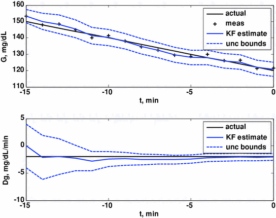
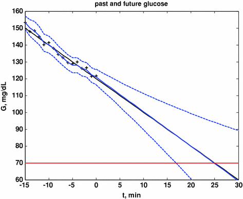
Fig. 2

Glucose (top) and rate-of-change of glucose (bottom). Actual (black), Kalman filter estimate (blue) and uncertainty bounds (–). The Kalman filter was initialized at t = −15 min, with uncertainty in the glucose and rate-of-change states. The estimated error variance improves with the measurement updates. Q = 0.01, R = 4. From Bequette [5]

Fig. 3

Actual glucose (black), measured (+), estimated (blue) and uncertainty bounds (–). The Kalman filter was initialized at t = −15 min. After t = 0 the estimated error variance grows since there are no measurements to improve the estimates. From Bequette [5]

Facchinetti et al. [25] have presented a two-state Kalman filter, which Bequette [5] has be shown to be identical to the 2-state model shown in Eq. (7).

The Kalman Filter estimates shown in Figs. 2 and 3 are based on a second-order (2-state) model. On the other hand, if it is assumed that the process noise drives the second derivative of glucose with time, the following third-order (3-state) model can be used:

$\Phi = \left[ {\begin{array}{*{20}c} 1 & 1 & 0 \\ 0 & 1 & 1 \\ 0 & 0 & 1 \\ \end{array} } \right],\quad \Gamma^{w} = \left[ {\begin{array}{*{20}c} 0 \\ 0 \\ 1 \\ \end{array} } \right],\quad C = \left[ {\begin{array}{*{20}c} 1 & 0 & 0 \\ \end{array} } \right],\quad x = \left[ {\begin{array}{*{20}c} g \\ d \\ f \\ \end{array} } \right],\quad y = G$

(15)

where g, d, and f, represent the glucose, rate-of-change of glucose, and the second-derivative of glucose with respect to time, respectively. In contrast to the two-state model in Eq. (7), an implicit assumption of this three-state model is that glucose rate-of-change tends to change at a constant rate for a period of time. This is equivalent to assuming that an automobile tends to maintain a constant acceleration for periods of time, subject to minor perturbations in the velocity. Naturally, this assumption will only hold for brief periods of time, such as when accelerating from, or braking before, a traffic light. The advantage of the 3-state model is that it captures dynamics near the maximum (peak) and minimum (valley) values of glucose. While the 3-state model yields better estimates for previous and current glucose estimates, Palerm and Bequette [37] found that the assumption of a constant first-derivative (2-state) for the future predictions led to better performance for multistep-ahead predictions on clinical data, than assuming a constant second-derivative (3-state).

Only gold members can continue reading. Log In or Register to continue