. A local cost c(x, u) is associated with each state x and action u. The aim of the AC algorithm is to minimize the average expected cost per state defined as
(1)
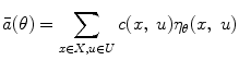
 . Define the value-function V θ (x) as the long-term expected cost when starting from state x and following control policy μ(u|x, θ). Function V θ (x) fulfills the following Poisson equation:
![$$\bar{a}(\theta ) + V_{\theta } (x) = \sum\limits_{u} {\mu (u|x,\;\theta )\left[ {c(x,\;u) + \sum\limits_{y} {p(y|x,\;u)V_{\theta } (y)} } \right]}$$](/wp-content/uploads/2017/04/A310669_1_En_4_Chapter_Equ2.gif)
(2)
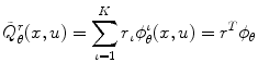
Similarly, define the action-value function Q θ (x, u) as the long-term expected cost starting at state x, taking control action u and following control policy μ(u|x, θ):
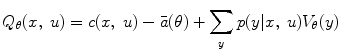
(3)

![$$\psi_{\theta } (x,\;u) = \nabla \ln \left[ {\mu (u|x,\;\theta )} \right]$$](/wp-content/uploads/2017/04/A310669_1_En_4_Chapter_IEq4.gif)
AC implementations may vary in the design of both the Actor and the Critic part. In most cases, the Critic estimates the Q-value function based on a function approximation method while the Actor follows a gradient descent approach for the iterative optimization of the control policy. A comprehensive review of RL and AC algorithms can be found in [20]. A scheme of a system controlled by an AC algorithm is shown in Fig. 1.
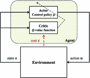
Fig. 1
System controlled by an AC algorithm
Critic: Policy evaluation. The critic evaluates the current control policy through the estimation of the Q-value function  . As (3) cannot be analytically solved in most cases, a function approximation method is usually employed in which
  is commonly approximated as a linear parameterized function of the form
where  ,
,  is a vector of basis functions dependent on the Actor’s parameters θ and
  denotes transpose. The method of Temporal Differences (TD) [21] is used for the update of the Critic’s parameter vector r and has the following general form
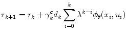
where the TD error d k , defined as the error between consecutive predictions, is given by the following formula

. As (3) cannot be analytically solved in most cases, a function approximation method is usually employed in which is commonly approximated as a linear parameterized function of the form(5)
, is a vector of basis functions dependent on the Actor’s parameters θ and denotes transpose. The method of Temporal Differences (TD) [21] is used for the update of the Critic’s parameter vector r and has the following general form(6)
(7)
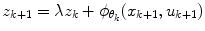
 is a positive non-increasing function which defines the learning rate of the Critic, 0 < λ < 1 is constant which stands as a forgetting factor. It is suggested in [21] that higher values of λ may result in improved approximations of the value function. A sequence of eligibility vectors z k is defined as
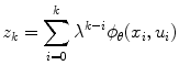
(8)
(9)
Thus, the final update procedure for Critic is formulated as
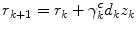
(10)
Finally, the average cost is updated as
![$$\bar{a}_{k + 1} = \bar{a}_{k} + \gamma_{k}^{c} \left[ {c(x_{k + 1} ,u_{k + 1} ) - \bar{a}_{k} } \right]$$](/wp-content/uploads/2017/04/A310669_1_En_4_Chapter_Equ11.gif)
(11)
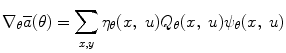
Actor: Policy improvement. The aim of the Actor is to minimize the average cost  through the iterative update of the control policy parameter vector θ based on the gradient
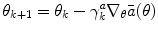
where  is a positive non-increasing function which defines the learning rate of the Actor. Based on (12), (4), and (5), the final update formula of the Actor policy parameter vector becomes
through the iterative update of the control policy parameter vector θ based on the gradient (12)
is a positive non-increasing function which defines the learning rate of the Actor. Based on (12), (4), and (5), the final update formula of the Actor policy parameter vector becomes(13)
3.2 AC-based Algorithm for Glucose Regulation
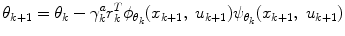
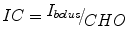
The AC algorithm implements a dual control policy for the optimization of the average daily BR and the IC ratio defined as:
where  is the insulin bolus dose and CHO is the amount of carbohydrates contained in a meal. The Critic estimates the Q-value function based on the TD method as previously described while the Actor updates the two control policies on a daily basis. The dynamics of the glucoregulatory system are represented as a MDP where the state and control action reflect the system’s status of one day. Define the glucose error EG as:
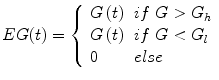
where  is the glucose value at time t and
 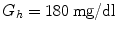 ,
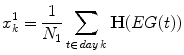
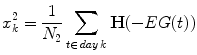
, 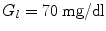 are the hyper- and hypoglycemia bounds respectively. The glycemic profile of day k is described by two features related to the hyperglycemic and hypoglycemic status of that day and more specifically to the average daily hypoglycemia and hyperglycemia error:
(14)
is the insulin bolus dose and CHO is the amount of carbohydrates contained in a meal. The Critic estimates the Q-value function based on the TD method as previously described while the Actor updates the two control policies on a daily basis. The dynamics of the glucoregulatory system are represented as a MDP where the state and control action reflect the system’s status of one day. Define the glucose error EG as:(15)
is the glucose value at time t and , are the hyper- and hypoglycemia bounds respectively. The glycemic profile of day k is described by two features related to the hyperglycemic and hypoglycemic status of that day and more specifically to the average daily hypoglycemia and hyperglycemia error:(16)
(17)
 is the Heaviside function and N i is the number of time samples above the hyperglycemia (i = 1) or below the hypoglycemia (i = 2) threshold. First, the features are normalized between [0 1]. The normalized features formulate the state
 ![$$x_{k} = [x_{k}^{1} \,x_{k}^{2} ]^{T}$$](/wp-content/uploads/2017/04/A310669_1_En_4_Chapter_IEq19.gif) of day k which is used by the algorithm for the estimation of the long-term expected costs and the control policies parameters. The control policy for the average BR and the IC ratio is updated as:
of day k which is used by the algorithm for the estimation of the long-term expected costs and the control policies parameters. The control policy for the average BR and the IC ratio is updated as: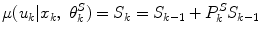
(18)
 is the rate of change of S k from day k − 1 to day k estimated as a linear combination of the features x:
(19)
A major challenge during the design of adaptive algorithms, especially for applications where safety matters, is to keep the learning period as short as possible. Furthermore, even during learning, the necessary safety constraints should be guaranteed. One way to achieve this goal in designing an AC-based algorithm is through the appropriate initialization of the policy parameter vectors θ S , which regulate the optimization of the control policy over time. The parameters θ S can be viewed intuitively as weights that define the percentage of change of the BR and IC ratio according to the daily hypoglycemia and hyperglycemia status. Setting these parameters away from their optimal values results in longer learning period, which can be crucial for the safety of the patient. One would expect that the percentage of change depends on the amount of information transfer (IT) from insulin to glucose in the sense that for high IT small adaptations of the insulin scheme may be sufficient whereas for low IT larger updates may be needed. Based on this reasoning, the IT from insulin to glucose has been estimated and used for the automatic, patient-specific initialization of θ S .
3.2.1 Automatic Tuning of the AC-based Algorithm
Assessing causality and IT between signals has been extensively studied and various measures have been proposed. A comprehensive review can be found in [22]. Transfer entropy (TE) is a powerful measure of IT, mainly due to its nonlinear and directional structure [23, 24], and has found promising application in biomedical signal analysis [25]. TE measures the information flow from a signal Y (source) to a signal X (target) while it excludes redundant effects coming from other signals. Let X = {xi, i = 1:n}, Y = {yi, i = 1:n} and Z = {zi, i = 1:n} be three observed random processes of length n. TE estimates the IT from process Y to X, which can be also translated as the amount of knowledge we gain about X when we already know Y, based on the following formula:
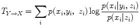
where  denotes probability density function (pdf) and log is the basis two logarithm. Division with the conditional probability of X to Z excludes the redundant information coming from both Y and Z without excluding, though, the possible synergistic contribution of the two signals on X [24]. Main challenge in computing (9) is the estimation of the involved pdfs. Several approaches have been proposed for this purpose [22]. One of the most commonly used methods is the fixed data partitioning in which the time-series are partitioned into equi-sized bins and the pdfs are approximated as histograms [26].
(20)
denotes probability density function (pdf) and log is the basis two logarithm. Division with the conditional probability of X to Z excludes the redundant information coming from both Y and Z without excluding, though, the possible synergistic contribution of the two signals on X [24]. Main challenge in computing (9) is the estimation of the involved pdfs. Several approaches have been proposed for this purpose [22]. One of the most commonly used methods is the fixed data partitioning in which the time-series are partitioned into equi-sized bins and the pdfs are approximated as histograms [26].TE was estimated as the IT from a delayed active insulin value to the current glucose excluding the dependence on the previous glucose value. In this case (20) takes the following form:
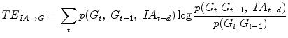
where G t is the current glucose value and IA is the insulin on board. The delay d in insulin was introduced in order to compensate on the physiological delay in insulin action due to absorption from the subcutaneous tissue to the blood and was chosen as d = 20 min. Expecting that high TE is related to smaller rates of change in the insulin scheme, the initial values of the policy parameter vectors  are set to be inversely proportional to the estimated TE per patient as:
where p denotes a specific patient and  is constant universally set as
  for the elements of
  related to hyperglycemia and
  for elements related to hypoglycemia.
(21)
are set to be inversely proportional to the estimated TE per patient as:(22)
is constant universally set as for the elements of related to hyperglycemia and for elements related to hypoglycemia.3.3 Results and Discussion
3.3.1 Simulation Environment
The AC-based algorithm has been in silico evaluated on 28 virtual T1D patients (10 adults; 10 adolescents; 8 children) using the educational version of the FDA-accepted University of Virginia (UVa) T1D simulator [27]. Two children have been excluded due to excessive glucose responses. The simulator comprises a database of in silico patients based on the meal simulation model of the glucose-insulin subsystem [28], a simulated sensor that replicates the typical errors of continuous glucose monitoring, and a simulated insulin pump. It allows for the creation of meal protocols and scenarios of varying insulin sensitivity (SI). Furthermore, the simulator provides optimized values for the BR and IC ratio which can be assumed as the standard SAP treatment of the patients as defined by his/her physician.
3.3.2 Meal Protocol
The meal protocol consisted of four kinds of meals: breakfast, lunch, dinner, and snack. In order to simulate the daily variation in terms of meal quantity and timing, the meal scenario per day was created in a randomized way as follows: each meal kind was assigned a range of possible quantities of grams of CHO and a range of timings as:
Breakfast: [30–60] g of CHO at [07:00–11:00]
Lunch: [70–100] g of CHO at [13:00–16:00]
Dinner: [70–110] g of CHO at [20:00–22:00]
Snack: [20–40] g of CHO at [23:00–00:00].
The accurate amount of grams of CHO and the timing for each meal and each trial day were chosen randomly from the respective ranges. As a second step, several dinners and snacks were omitted in order to represent the common case of missing these meals. The missed meals were randomly distributed within the trial days. The average duration of each meal was considered 15 min and the meals were announced to the controller 30 min prior to intake.
In order to simulate the errors when real patients estimate the CHO content of their meal, a random meal uncertainty uniformly distributed between −50 and +50 % has been introduced. The total trial duration was 10 days. The initial values of BR and IC ratio have been set equal to their optimized values as provided by the UVa simulator. For adults and adolescents, these values are close to the optimal ones, whereas in the case of children they are too high and, when applied in an open-loop scenario, they lead to excessive insulin infusion and frequent hypoglycemic events [15]. Consequently, the AC algorithm must perform significant updates of the BR and IC ratio in order to optimize glucose regulation, a fact that renders the duration of the learning period in children very challenging.
Three different initialization scenarios of the policy parameter vectors  have been investigated:
have been investigated:
S1. The policy parameter vectors are initialized to zero values.
S2. The policy parameter vectors are initialized to random values with magnitude ranging in (0, 1).
S3. The policy parameter vectors are initialized based on the estimated insulin-to-glucose transfer entropy per patient as in (22).
The Control Variability Grid Analysis (CVGA) [29] has been used for the evaluation of the AC algorithm, while the risk of hypoglycemia has been estimated based on the Low Blood Glucose Index (LBGI) [30].
Figure 2 presents the CVGA plots for all patients and scenarios S1–S3. Table 1 presents the percentage of values within the A + B zones of the CVGA separately for each age group and the three scenarios. Setting the maximum acceptable duration of the learning period to five days, these results refer to the last five days of the trial. Finally, the daily evolution of the LBGI for the three groups when following scenarios S1–S3 is presented in Fig. 3. This result refers to the total trial duration.
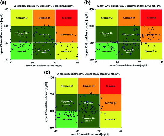
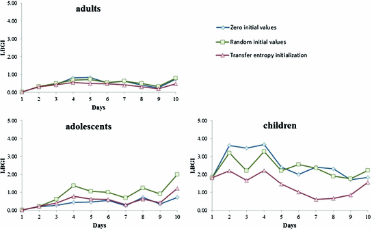
Fig. 2
CVGA plots for all patients and the last five trial days when AC initialization is based on scenario (a) S1, (b) S2 and (c) S3
Table 1
Percentages (%) in the A + B zones of the CVGA for the three age groups and scenarios S1, S2, S3
Patient age group | S1 | S2 | S3 |
|---|---|---|---|
Adults | 93.00 | 95.00 | 98.00 |
Adolescents | 88.00 | 78.00 | 90.00 |
Children | 41.00 | 41.00 | 73.00 |
Fig. 3
Evolution of LBGI during the 10 days of the in silico trial for adults, adolescents and children and scenarios S1 (blue), S2 (green) and S3 (red)
Figure 2 shows that, when the AC initialization is based on the patient-specific TE (S3), the general performance of the algorithm after five days of learning is increased with 89 % of the values in the A + B zones of the CVGA, compared to 78 % for scenario S1 and 73 % for S2. The same result can be observed from Table 1, where the values are separately presented for each patient group. Furthermore, from Table 1 it is clear that most of the hypoglycemic events present in Fig. 2 belong to the age group of children. This is expected since, as mentioned earlier, the initial simulator-suggested values of BR and IC ratio are far from being optimal. The contribution of the TE-based tuning especially in the case of children is thus critical as it significantly reduces the duration of the learning period and achieves increased overall performance. Figure 3 supports this above remark presenting the evolution of the daily LBGI over the total trial duration. As expected, children start from much higher LBGI values compared to adults and adolescents. It can be further seen that the daily LBGI is kept to low and comparable values among the three scenarios for adults and adolescents, however, in the case of children, LBGI reduces much faster when the AC algorithm is initialized based on the TE compared to the zero or random initialization.
Related posts:
 Models for In-Silico Evaluation of Closed-Loop Insulin Delivery Systems in Type 1 Diabetes
Parameters Describing Gut Absorption and Lipid Dynamics in Relation to Glucose Metabolism During a Routine Oral Glucose Test
Modeling of the Dynamic Effects of Free Fatty Acids on Insulin Sensitivity
Modeling of Diabetes Progression
Prevention Using Low Glucose Suspend Systems
and Minimal-Type Compartmental Insulin-Glucose Models: Theory and Applications
Models for In-Silico Evaluation of Closed-Loop Insulin Delivery Systems in Type 1 Diabetes
Parameters Describing Gut Absorption and Lipid Dynamics in Relation to Glucose Metabolism During a Routine Oral Glucose Test
Modeling of the Dynamic Effects of Free Fatty Acids on Insulin Sensitivity
Modeling of Diabetes Progression
Prevention Using Low Glucose Suspend Systems
and Minimal-Type Compartmental Insulin-Glucose Models: Theory and Applications
Stay updated, free articles. Join our Telegram channel

Full access? Get Clinical Tree


