where p1, p2 and p3 are three positive parameters. The model is very simple and each term on the right-hand side would appear to make sense: variations of glycemia are due, first, to the level of glycemia itself (the higher the glycemia, the faster its decrease); second, to insulinemia (the higher the insulinemia, the faster the decrease in glycemia); and, third, some necessary glucose production (say, by the liver), which we may assume constant throughout a short experiment.
The qualitative analysis of the model reveals however that negative solutions are permissible: at zero glycemia, its derivative may well be strictly negative, depending on the level of insulinemia.
The fact that solutions of the model, i.e. predicted glycemia, can be negative is evidently contrary to common sense. There are then at least two possible philosophical stances, which the modeller can take in the face of such paradoxical result. The first is to assert that the model has some limited validity in some circumscribed region of its state space: in the present case, that the model is still good, if insulin is not too high and glycemia is not too low. Oftentimes, modellers subscribing to this philosophical position defend it by quoting G.E.P. Cox: “Essentially, all models are wrong, but some are useful” [23]. We believe this position to be somewhat simplistic, and potentially misleading: it aggregates all models, irrespective of their merits, into the class of “wrong” models, and elects a model as ‘appropriate’ depending merely on contingent utility. We may offer a two-tiered philosophical approach, by defining a model to be “inconsistent” when it does not agree with irrefutable available data, and further by defining a model as “obsolete” when it is inconsistent and another model exists, which does explain the irrefutable available data. If the qualitative behaviour of a model’s solutions contradicts common knowledge, then the model’s construction must imply some fundamental mistake: for example, from the very moment that Bolie’s model was published, it was clear that it could predict glucose concentrations to become negative, hence it was inconsistent from the very start. However, at the time it was not obsolete, because no other model existing at the time (there were none) was consistent: indeed, Bolie’s model spurred mathematical investigation of the Glucose-Insulin system, and deserves our affection and respect for having been a pioneer. The fundamental mistake of Bolie’s model concerns the form of the second term, the decrement in glycemia depending on insulinemia. Figure 1 summarizes the problem: the model asserts that, no matter how little glucose there is in blood (even zero), we would be able to make the tissues extract as much glucose as we want, just by increasing insulin levels. Since we cannot take out of plasma the glucose that is not there, the second term in Bolie’s model is wrong and determines in fact the possible negativity of predicted glycemia.
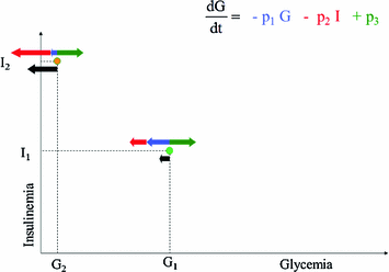

Fig. 1
Schematic representation of Bolie’s model behaviour. Black arrows represent the variation in blood glucose concentration as a result of glucose tissue uptake mediated by insulin (red arrows), glucose produced by liver (green arrows) and spontaneous glucose elimination. While the model works correctly around the point (G1, I1), when plasma glucose is low and serum insulin is high (G2, I2) the model would predict negative glycemias, by still (incorrectly) allowing arbitrarily high glucose extraction
A consequence of flawed model construction, as detectable by theoretical behaviour inconsistent with basic observations, is that the parameters of the model may well be devoid of meaning, in so far as they refer to phenomena which either do not exist or are incorrectly represented in the model. For example, the insulin-dependent glucose elimination rate p2 in Bolie’s model, which would quantify the number of mM/min of glycemia decrement per pM of insulin concentration, has no meaning: insulin-stimulated glucose uptake has some value at high glycemia and is in fact zero at zero glycemia, so that giving it a single value over the entire allowable range of glycemias is, at a minimum, misleading.
It is clear that models capture only certain features of the phenomenon under investigation, and that ultimately all models will fail to agree with data from sufficiently advanced and detailed experiments. All models are simplifications of reality, will eventually be proven inconsistent by further experimentation, and will eventually be made obsolete by better models.
When designing a new model to interpret a physiological phenomenon, studying the qualitative properties of the solutions ensures that the model is not already inconsistent at the moment it is proposed. As another example from the literature on the IVGTT we may mention the Minimal Model [21], which is still the most widely employed model to assess insulin resistance, even in recent research applications [24–31]. This model describes the time-course of glucose plasma concentrations, depending upon serum insulin concentrations and on a variable X, representing the ‘Insulin activity in a remote compartment’ [32]. While in later years different versions of the Minimal Model appeared [33, 34], the following discussion refers to the original formulation [21, 35] as presented in [36] with detailed instructions on how to identify the model from data.
A formal, qualitative study of the solution of the model appeared in the year 2000 [37]. The model is non-autonomous, and it can be proven that, mainly depending on the non-autonomous time term, when glucose concentrations are higher than a threshold value (lower than observed basal glycemia) the variable X goes to infinity and the system does not admit an equilibrium. Proponents of the model specifically state that the model is ‘valid’ only for the 3 h or so of duration of a typical IVGTT: on the other hand the Insulin Sensitivity index, as derived from the model, is defined for time that goes to infinity. Figure 2, panel b (dotted lines) shows the anomalous behaviour in the insulinemia predictions which are visibly increasing at the end of the observation period and which would be predicted to increase to extremely high levels within a few hours instead of tending to the equilibrium value corresponding to basal insulin concentration IBb.
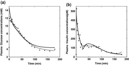

Fig. 2
Glucose and Insulin predictions with the SDM and MM models. Panels a and b respectively show observed plasma glucose concentrations and observed plasma insulin concentrations (asterisks) following an IVGTT experiment, along with predictions by the Single Delay Model (continuous lines) and by the Minimal Model (dotted lines)
We find ourselves in essentially the same situation as with Bolie’s model: in that case, solutions could become negative, in this case solutions can explode to infinity. Limiting the operation domain of Bolie’s model to not-too-high insulinemias, or limiting the operation domain of the Minimal Model to ‘about three hours’ does not address the issue, which is that if an abnormal behaviour is produced by the model this means that the model’s construction incorporates flawed assumptions. Both models therefore could have been diagnosed as inconsistent from the start. It remains to be seen if they are now obsolete.
Recent work [22] presented in fact an alternative model for the interpretation of glucose and insulin concentrations observed during an IVGTT: the so-called discrete Single Delay Model (SDM). In the context of the present discussion, the relevant thing to notice is that this model has been proven to have solutions mathematically consistent with expected behavior [38], admitting the fasting state as its single equilibrium point and converging back to it from the perturbed state. Moreover, the model aimed at being consistent with known physiology by incorporating a limited pancreatic insulin secretion in response to increasing glucose concentrations: Fig. 2 (continuous line) reports the fitting of the SDM over an IVGTT experiment. While no claim is made as to the optimality of the SDM in any sense (indeed, better models are expected to be formulated in the future), its existence makes the other two models obsolete, in the sense defined above.
Model builders should therefore study the qualitative behaviour of the solutions of their models in order to assure that these are capable of describing consistently the relevant physiology, as a pre-condition to obtaining reliable quantitative estimates of the parameters of interest.
4 Second Pitfall: Using Interpolated Noisy Observations as Input Functions, Particularly When Fitting Coupled Systems
The idea that interpolated observed data, used in place of theoretically reconstructed curves, are a reliable approximation of the true signal for the purpose of parameter estimation is rather widespread in the domain of insulin glucose model (ex multis [36, 39]).
What is generally not considered is that, during an estimation process for models depending on input or forcing functions, the optimizer algorithm attempts to obtain the best possible reconstruction of the output signal changing the parameter values conditional on the input signal. This determines, in particular, the possible leverage of accidental data oscillations in the input signal, through ad–hoc parameter values, in order to build an output signal that matches output observations. The result is, indeed, an apparently good match to the observed output, and what is sometimes not appreciated is that this apparently good fit is contingent on finding parameter values exploiting accidental variations in input: the result is artifactual because it does not build on the expected behavior of the model but on stochastic realizations of the errors; it is inherently non-reproducible, because the parameters found depend directly on such random variations in input; and the corresponding parameters have a high variability, because different random configurations of the input will produce in general different parameter values attempting to reconcile the variable input with the output observations.
As a clear example of the misleading results that can be obtained when incurring in the pitfall of using interpolated observations as input into the model, consider once again the Minimal Model of glucose-insulin dynamics, in the form and with the estimation procedure proposed in 1986 [36]. In this case, two sub-models are used, one for glucose kinetics depending on insulinemia as driving function, and one for insulin kinetics depending on glycemia as driving function: the proposed estimation procedure consists of using observed insulinemias to represent the true input for the purpose of estimating glucose kinetics and then using observed glycemias for the estimation of insulin kinetics (instead of performing a single optimization on both feedback control arms of the integrated glucose/insulin system). Following this approach, the estimated parameters are optimal in predicting observed glucose assuming the erratic observed insulin as the true value of the insulin concentration (and viceversa), but would not be optimal in describing the modeled effects of expected glucose on expected insulin and viceversa. This fitting strategy produces sets of estimated parameters such that the expected time course of glucose using the expected time course of insulin as input may differ markedly from both the actual glucose observations and from the expected glucose obtained using the noisy insulin observations as input. In other words, this strategy produces parameter values which do not make model predictions of glucose and insulin consistent with each other. Furthermore, the exploitation of random variations in input determines the very ability of the algorithm to reproduce characteristic features of the output signal, which the model may have difficulty reproducing when moving from the theoretical or expected input signal.
Stay updated, free articles. Join our Telegram channel

Full access? Get Clinical Tree


