1.3 Statement of the Problem
The development of a safe predictive and advisory system, such as the DIAdvisorTM tool, would require patient-specific dynamical models of the glucose metabolism able to describe the blood glucose evolution based on the most significant inputs, namely, meal carbohydrates, exogenous injected insulin and possibly energy expenditure due to physical activity [60] to be used in a model predictive control setup [44]. Characteristics required in such models include a good trade-off between simplicity and accuracy, stability, qualitative correct responses to inputs and predictive capabilities with particular emphasis on hypo- and hyperglycemia detection. In addition, predictors targeting blood glucose forecasting need to be developed in parallel, as well.
Motivated by the above, this contribution addresses the questions of how to identify personalized models from individual patient data and how to provide individualized short-term blood glucose predictors.
1.4 Inherent Challenges in T1DM Modeling
Despite significant efforts devoted to the problem of blood glucose regulation in type 1 diabetic patients over the last decades (see e.g. [15] for a comprehensive review), many inherent challenges that must be overcome still remain. At the most basic level, the disease can be viewed as a process having one output, namely, glucose concentration in plasma, and two inputs, namely, meal carbohydrates and administered insulin. The first and perhaps most crucial challenge to overcome in modeling is that of poor data excitation: often the inputs are simultaneous and in the same ratio, the so-called insulin-to-carbohydrate ratio, precluding the possibility of distinguishing their relative effects. It is still an open issue how to strongly excite the system in order to obtain data meaningful for identification purposes preserving at the same time the patients from the risk of serious clinical events. Second, the most widespread way of treating diabetes comprises a series of impulse-like control actions, i.e., insulin injections and food intakes, applied several times during the day at irregular sampling instants, typically at wake up, meal and bed times, the decisions being based on scarce assays of the controlled variable, i.e., blood glucose. This rises the problem of non-uniformly sampled and infrequent data and, since the signals in play interact in the bloodstream, introduces assumptions on the subcutaneous-to-intravenous insulin absorption and gastro-intestinal carbohydrates absorption dynamics.
In the last ten years, advances in sensor technology saw the advent of continuous glucose monitors (CGM), systems capable of measuring glucose concentration frequently (e.g., every 5 min) for several days, providing the patient with well-sampled data in real time. However, it is important to stress that together with the benefits, they introduce yet another limitation. Indeed, those devices measure glucose concentration in the interstitium and not in plasma. Interstitial glucose (IG) fluctuations are related to BG presumably via diffusion process [37, 63]. This leads to a number of issues, including distortion (which incorporates a time lag) and calibration errors, and necessitates the development of methods for their mitigation. In particular, it is necessary to consider that, since the BG-to-IG kinetics act as a low-pass filter, the frequency content of interstitial glucose is different from that of blood glucose [9, 47].
As for the inputs, when taking into account the appearance of insulin in the bloodstream from subcutaneous delivery and that of glucose in plasma after a meal, new time-lags and dynamics are introduced; further, subcutaneous insulin infusion involves degradation at the site of delivery. In addition, meals must be recorded by the patients, and the actual amount of carbohydrates must be estimated, a process that is prone to errors. Also, in practice, the combination of simple and complex carbohydrates, fats and proteins can affect the glucose absorption in the digestive system. Unrepresented inputs, such as stress and illness constitute another challenge to diabetes modeling. Furthermore, it is a well known fact that physical activity, apart from having a glycemia-lowering effect due to utilization of glucose by the muscle cells, enhances insulin sensitivity, playing a substantial role in the picture, but the magnitude and duration of such effects are hard to consider. Another important aspect is the degree of variability of the overall system dynamics over the day (the so-called “dawn phenomenon”, for instance, is characterized by increased insulin resistance during the morning hours [70]).
A priori knowledge of the diabetes process indicates two fundamental properties that should be satisfied by any sound and valid model:
the gain associated with the insulin input should be negative (i.e., an increase in insulin results in a decrease in glucose concentration)
the gain associated with the meal input should be positive (i.e., a meal results in an increase in glucose concentration).
However, the values of the above mentioned gains are related to age of the subject, disease duration, body mass index (BMI), insulin sensitivity, β-cells responsiveness and probably many more unknown factors so that it is not clear how to take them into account in the modeling process.
1.5 Models in Diabetes
In diabetes research and therapy, modeling of the glucose-insulin control system has received significant attention for more than 40 years [15]. Several types of models serving different purposes were proposed, most of these efforts being first-principles based descriptions of the physiological relationships associated with T1DM, and only to a lesser extent mathematical modeling by means of system identification.
1.6 Physiological Models
The first pioneering work describing the relationships between insulin and glucose utilization was that of Bolie [7], later modified by Ackerman and McGucking [2] in order to provide a model of the glucose metabolism during an oral glucose tolerance test (OGTT). Greater attention was received by the so-called minimal model [5, 6], developed for the specific purpose of quantifying pancreatic responsiveness and insulin sensitivity during an intravenous glucose-tolerance test (IVGTT) in non-diabetic individuals. The model consists of three differential equations describing plasma glucose and plasma insulin in a remote compartment, accounting for neither the dynamics of subcutaneous insulin infusion nor the dynamics of gut glucose absorption from a carbohydrates meal. In [40], a simulation model was presented, and later validated on a set of 24 subjects [41]. Glucose-insulin pharmacokinetics/pharmacodynamics in non-diabetic subjects was described by a 19-state model developed by Sorensen [57], the major shortcoming of this model being the failure in capturing the hyperglycemic events characteristic of type 1 diabetes [43]. The nonlinear model proposed by Hovorka et al. [35] describes glucose-insulin dynamics with several differential equations in three subsystems: a glucose subsystem, an insulin subsystem and an insulin action subsystem. Model inputs are the rate of subcutaneously infused fast acting insulin, meal carbohydrates amount and time of ingestion and its outputs are plasma glucose and insulin concentrations. The absorption kinetics associated with subcutaneous insulin delivery of the above mentioned model was later modified [69], the model replacing the original subcutaneous insulin subsystem consisting in two parallel fast and slow channels for insulin absorption as well as a degree of insulin degradation at the injection site, and integrated in a simulation environment dedicated to closed-loop evaluation of insulin delivery systems [68]. The efforts by Dalla Man and co-workers presented in [16–18, 20] lead to the meal simulation model of the glucose-insulin system [19] which has been accepted by the Food and Drug Administration (FDA) to be used as a substitute for animal trials in preclinical tests of closed-loop development [38, 39]. Dalla Man and co-workers [19] used a sophisticated triple tracer method to estimate important meal-related quantities such as the rates of appearance of glucose in the blood from the meal, endogenous glucose production, utilization of glucose, and insulin secretion. Reviews of physiological diabetes models include that of Nucci and Cobelli [49], who specifically examined several models of subcutaneous-to-intravenous insulin kinetics, Makroglou and co-workers [45] presenting an overview of existing software packages specific to diabetes modeling and finally Cobelli and co-workers [15], discussing the main contribution to both modeling and control in diabetes from the early 1960s.
1.7 Predictive Models
Although seemingly simple in concept, the problem of glucose prediction in an active individual has to date proved intractable. Currently, continuous glucose monitoring (CGM) devices are the available technology able to provide high/low glucose alarms when certain user specified preset threshold levels have been crossed and to deliver warnings of events that are likely to occur if the current trend continues. However, patients will benefit more from an early alarm that predicts the hypoglycemic episode before it occurs. A review of hypoglycemia prevention algorithms is reported in [4]. To date many studies have investigated the possibility of predicting blood glucose concentration for the purpose of regulating glucose intervention, in order to enable individuals to take corrective actions and avoid low or high glucose values. Bremer and Gough [8] originally developed the idea of T1DM CGM time-series analysis using 10 min sampled data from ambulatory T1DM patients to identify autoregressive (AR) models. They explored 10, 20 and 30 min prediction horizons, and report that the 10 min predictions are accurate and the 20 or 30 min predictions may also be acceptable for a limited set of data only. However, no quantification of the accuracy of the model predictions was provided. In [55] tenth-order autoregressive models were identified from 5-days long glucose time-series belonging to a population of five in-hospital subjects. Performances of a single, cross-subject model compared with individual models were evaluated on 30 and 60 min prediction horizons. Gani et al. [30] used a 30th-order AR model with data smoothing and a regularization procedure to minimize the changes in the glucose first-derivative, reducing the prediction lag for 60 and 90 min-ahead prediction compared to [55]. Sparacino et al. [59] collected 48 h of continuous (3 min) glucose data from 28 T1DM subjects in ambulatory conditions. In their retrospective analysis, they recursively identified simple polynomial and AR models from the CGM time-series data, prefiltered to removed noise spikes. They investigated prediction horizons of 10 and 15 steps (i.e., 30 and 45 min) and concluded that hypoglycemia can be detected 25 min before the hypoglycemic threshold is passed. In [51] a Kalman filter approach was proposed, which only used information on past CGM readings by assuming a double integrated random walk as prior for glucose dynamics and estimating the states corresponding to the interstitial glucose level, and the first and second derivative thereof, i.e., rate of glucose change and acceleration. The method was evaluated for 13 hypoglycemic clamp data sets in [50]. Using a hypoglycemic threshold of 70 [mg/dL], the sensitivity and specificity were 90 and 79 %, respectively, with unknown alarm time. A tutorial overview of algorithms for CGM time series analysis to the purpose of alarm generation is provided in [58]. Eren-Oruklu et al. [23] proposed a recursive second-order AR and ARMA model identification strategy with an adjustable forgetting factor for healthy and type II diabetics. Their models utilized only recent glucose history from a CGM device, achieving 3–5 % error for 30 min ahead prediction. In [48] a kernel-based regularization learning algorithm, in which the kernel and the regularization parameter are adaptively chosen on the basis of previous similar learning tasks, using past glucose information, was presented. The past few years witnessed the investigation of neural networks (NN) models for short-term glucose prediction proving it to be a competitive approach. Pappada et al. [54] created NN models with variable predictive windows in the range 50–180 min, trained using 18 patients CGM datasets and evaluated on patient data not included in the neural network formulation. They concluded that their models performed adequately in the normo- and hyperglycemic ranges, whereas hypoglycemic events were overestimated, a potential reason for that being due to the minimal occurrences of hypoglycemia in the training data. In [25] a feed-forward NN whose inputs were CGM samples in the previous 20 min and the current time instant, and whose output was the glucose concentration 15, 30 and 45 min ahead was tested on 15 actual data sets. The root-mean-squared error (RMSE) was 10, 18 and 2 [mg/dL] for the 15, 30 and 45 min prediction, with a delay of around 4, 9, and 14 min for upward trends, and 5, 15, and 26 min for downward trends. Dassau and co-workers [17] developed a real-time hypoglycemia prediction suite combining five individual algorithms, namely, linear prediction, Kalman filtering, hybrid impulse response (HIIR) filtering, statistical prediction and numerical logical into a voting-based system to predict hypoglycemia from 1 min sampled CGM data. A 35 min prediction horizon with an alarm threshold of 80 [mg/dL] and a voting threshold of three to five algorithms to predict hypoglycemia resulted in a 91 % correct predictions. A short-coming of the methods listed above is the lack of exploitation of the dynamic interplay between previously injected insulin, meal intake and eventually exercise to the purpose of improving glucose prediction. Hovorka and his group [35] performed experiments with ten T1DM patients under clinical conditions, using their physiological model to make predictions of glucose data up to 60 min into the future. The glucose was measured intravenously, but delayed by 30 min to mimic subcutaneous measurement. The model parameters were recursively estimated using a Bayesian method. The predictions of the resulting models had RMSE values of 8.6, 13.0, and 17.3 [mg/dL] for 2, 3, and 4-step (i.e., 30, 45, and 60 min) predictions, respectively. Finan et al. [27] analyzed both batch-wise and recursively identified patient-specific ARX models for 9 patients with a mean 30 min prediction error RMSE of 26 [mg/dL]. An ARX model with a nonlinear forgetting factor scaled according to the glucose range was considered in [11, 12], and a 45 min prediction horizon showed good results. Finally, in [31] it was asserted that a universal data-driven model identified from CGMS time-series from a patient applying the algorithm previously published by the same authors in 2009 [30] could be used to make near-future glucose concentration predictions for other patients without any model customization procedure. They used regularization techniques to filter data from 34 subjects, then, using the filtered data, they develop auto-regressive models of order 30 to the purpose of making short-term, 30-min-ahead predictions. A feed forward NN was also exploited in [54] and tested on 10 real datasets, incorporating, in addition to CGM data, other inputs such as SMBG readings, information on insulin, meal, hypo- and hyperglycemia symptoms, lifestyle, activity and emotions and predict glucose values up to 75 min. In [71–73], 30-min-ahead prediction was performed with a feed-forward NN in cascade with the first-order polynomial model in [59]. The inputs to the linear predictor were the past CGM values weighted using a forgetting factor, while the inputs to the NN were current CGM and its trend, information on the past error committed by the polynomial model and information on meal, supplied as plasma glucose rate of appearance obtained from the physiological model of [19]. Zhao et al. [74] used a latent variable-based approach to predict future CGM values from past CGM and known carbohydrate and insulin boluses, transformed into time-smoothed inputs using second-order transfer functions. The method was applied to collected clinical data and simulated data generated by the model described in [38, 39]. They concluded that their LV-based method resulted in models whose prediction accuracy was as least as good as the accuracies of standard AR/ARX models. In [24] a multi-sensor body monitor providing seven signals related to activity and emotional conditions was used in addition to a CGM monitor to improve glucose prediction. A multivariate ARMAX model with weighted recursive least-squares estimation of the unknown parameters using a variable forgetting factor was proposed. Results showed that the prediction error is significantly reduced with the addition of the vital signs measurements, as compared to an ARMA model based only on CGM signals.
2 Experimental Conditions and Clinical Data Acquisition
In the framework of DIAdvisor™ [22], acquisition of bioclinical data linked or potentially involved in blood glucose control from insulin-treated diabetic subjects was accomplished in a series of experimental sessions. The investigations focused on a population of basal-bolus regimen treated subjects, either as combination of multiple daily insulin injections (MDI) including long-acting and fast-acting analogues or as continuous subcutaneous insulin infusion (CSII) of fast-acting analogues from a pump. The clinical study was performed at the Clinical Investigation Center CIC-CHU in Montpellier, France. Collected data include: specific patient parameters (e.g., gender = male, age = 43 years old, BMI = 23.7, weight = 67 kg), characteristics related to diabetes (e.g., disease duration = 10 years, insulin delivery = external pump), associated health conditions and therapies, food intakes and administered insulin doses registered in a logbook, capillary glucose strips, interstitial glucose levels, plasma glucose and plasma insulin concentrations from drawn blood samples as well as vital signs.
2.1 Equipment
For the whole duration of the study, the subjects were equipped with state-of-the-art devices provided by the DIAdvisor™ Consortium complying with the study protocol as explained in the following subsections.
2.1.1 HemoCue™ Glucose Analyzer
The HemoCue™ Glucose Analyzer [34] is a blood glucose meter based on a glucose dehydrogenase method and consisting of a pocket size handheld analyzer and a unique disposable microcuvette. The analyzer was factory calibrated and no calibration was needed between cuvette batches. The device was used by each patient as a reference glucose meter, assessing plasma glucose levels from finger-stick samples.
2.1.2 Abbott Freestyle Navigator™
The Abbott Freestyle Navigator™ [1] is a Continuous Glucose Monitoring System (CGMS) consisting of an amperometric electrochemical sensor placed under the skin, a wireless transmitter connected to the sensor and a wireless receiver collecting the sensor signals. The subcutaneous sensor was inserted about 5 mm into the subcutaneous tissues and could be worn for up to five days before replacement. Calibration relative to capillary glucose was required at specific times, namely, 10, 12, 24 and 72 h after insertion. Using the WIRED ENZYME™ technology, the sensor converted glucose concentration to electrical current. Once every minute the transmitter sent the estimate of the interstitial glucose concentration to the receiver, which displayed the final values once every 10 min.
2.2 Study Protocol and Experiments
The clinical study consisted of three visits: Visit 0 for patients screening, Visit 1 for sensors initialization and Visit 2 for 75 h in-hospital tests. Figure 2 gives the flow chart of the trial.


Fig. 2
DIAdvisor™ Data Acquisition Trial. Visit 0 Screening visit (green box), Visit 1 sensor initialization visit (blue box), Visit 2 in-hospital tests (red box)
2.2.1 Visit 0
Prior to any study-related procedure, the purpose of this visit was to perform a screening examination of the patient, the outcome of it being recorded in the clinician’s sheet.
2.2.2 Visit 1
Within 4 weeks of visit 0 the patient was admitted at the clinic to initialize the Abbott Freestyle Navigator™ device. The sensor was inserted subcutaneously into the patient’s skin and calibrated against capillary glucose by a nurse. The subject was hospitalized at best 48 h after sensor insertion, in order to begin the tests with a well-calibrated device.
2.2.3 Visit 2
During the whole 3-days-long visit, the patient was permanently equipped with the Abbott Freestyle Navigator™ [1] device. Standard meals for breakfast (8:00 a.m.), lunch (1:00 p.m.) and dinner (7:00 p.m.) were served, the amount of administered carbohydrates being 42, 70 and 70 g, respectively. Blood samples were collected by nurses to measure plasma glucose and plasma insulin concentrations: every hour during day, every 2 h during night, every 15 min after meals for 2 h. A specific sampling scheduled was adopted after breakfasts: 30 min before, mealtime, 10, 20, 30, 60, 90, 120, 150, 180, 240 and 300 min after, for a total of 37 blood samples per day. No specific intervention on usual diabetes treatment was scheduled during the period. The patients decided their insulin needs according to the HemoCue™ Glucose Analyzer [34] measurements as usually in activities of daily life. Throughout the chapter, modeling results obtained with visit 2 data will be presented.
2.3 Patients Selection Criteria
A total of 30 diabetic subjects, male and female adults, were included in the study to allow availability of data from a wide spectrum of patients under basal-bolus regimen. Among these, a population of nine patients was chosen, the selection criteria being the quantity of data collected during visit 2 (>80 % of the expected), no sensor failures and logbook correctly filled in. Exclusion criteria were data partially collected, laboratory results not available and/or patients not observant in annotating insulin/meal intakes. Table 1 reports the characteristics of the selected patients. Data from a representative patient are shown in Fig. 3.
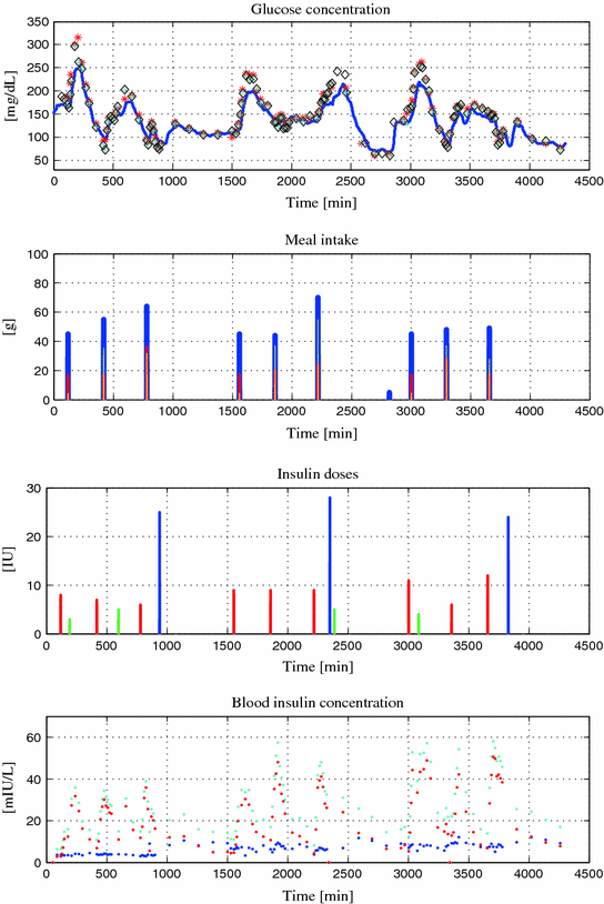
Table 1
Patient characteristics
Patient ID | Insulin therapy | HBA1c [%] | BMI |
|---|---|---|---|
102 | MDI | 6.5 | 26.5 |
103 | CSII | 9.1 | 23.7 |
104 | MDI | 7.6 | 20 |
105 | CSII | 7.8 | 24.1 |
106 | CSII | 7.8 | 21.2 |
107 | CSII | 8.9 | 25.3 |
115 | MDI | 8.5 | 19.7 |
120 | MDI | 9 | 22.4 |
130 | MDI | 8.8 | 29.4 |

Fig. 3
Patient CHU0102 data versus Time [min]. Top Glucose concentration [mg/dL]: interstitial (blue), plasma (red), finger stick (cyan and black); Upper Center Meal intake [g]: carbohydrates (blue), lipids (red), proteins (yellow); Lower Center Insulin doses [IU]: basal (blue), bolus (red), correction (green); Bottom Blood insulin concentration [mIU/L]: basal (blue), bolus (red), total (cyan)
3 Modeling of the Gluco-Regulatory System
The physiology of glucose metabolism in diabetes can be thought of as having one output, i.e., glucose level in the bloodstream y BG , and two main inputs, i.e., carbohydrate intake u carb and administered insulin I ir . Further, given that physical activity has been proven to decrease plasma glucose levels due to increased glucose uptake by the exercising muscles [70], the effect of exercise, i.e., increased heart rate, respiration rate and body movements, is therefore to be regarded as an additional input or load disturbance. Hence, for modeling purposes, based on current knowledge of the overall physiological model, four subsystems have to be considered (Fig. 4):
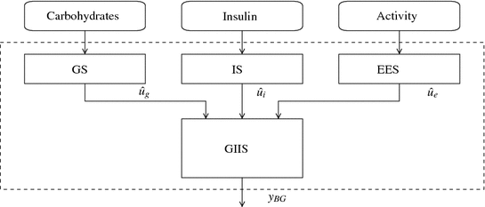
the glucose subsystem (GS), describing glucose intestinal absorption following a food intake;
the insulin subsystem (IS), accounting for the pharmacokinetics of the exogenously administered insulin;
the physical activity and energy expenditure subsystem (EES), measuring the rate of physical activity intensity;
the glucose-insulin interaction subsystem (GIIS).

Fig. 4
Physiological model describing diabetic blood glucose dynamics. Notation: GS glucose subsystem, IS insulin subsystem, EES energy expenditure subsystem, GIIS glucose insulin interaction subsystem; û g glucose rate of appearance following a meal, û i insulin in plasma after subcutaneous injection, û e energy expenditure, y BG blood glucose
In this chapter, compartment models from the literature are exploited to describe the GS and IS. Data-based system identification is used, instead, to model the GIIS.
3.1 Glucose Subsystem
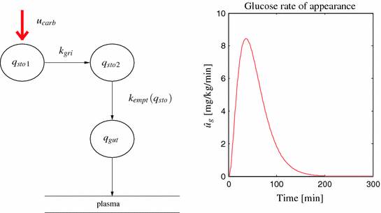
Glucose transit through the stomach and upper small intestine was described by a nonlinear chain of three compartments, where the first two compartments represent the stomach (solid and liquid phases) and the third one depicts the intestine. The left plot in Fig. 5 illustrates the model. Equations are [16]:
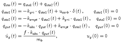
where  [mg/kg/min] denotes the rate of appearance of glucose in plasma, q sto1 and q sto2 [mg] are the amounts of carbohydrates in the stomach (solid and liquid phase, respectively), u carb [mg] is the amount of ingested carbohydrates, q gut [mg] is the carbohydrate mass in the intestine, k gri is the rate of grinding, k empt the rate of gastric emptying, m b [kg] the subject’s body weight, k abs the rate of absorption and f the fraction of intestinal absorption that actually appears in plasma. The rate of gastric emptying was a non-linear function of the amount of carbohydrates in the stomach q sto according to the following relationship:
![$$\begin{aligned} k_{empt} \left( {q_{sto} } \right) & = k_{min} + \frac{{k_{max} - k_{min} }}{2}. \\ & \left\{ {\tanh \left[ {\alpha \left( {q_{sto} - b \cdot D} \right)} \right] - \tanh \left[ {\beta \left( {q_{sto} - c \cdot D} \right)} \right] + 2} \right\} \\ \end{aligned}$$](/wp-content/uploads/2017/04/A310669_1_En_9_Chapter_Equ2.gif)

Dalla Man and co-workers provided us with the mean population values for the parameters appearing in Eqs. 1, 2, 3 used throughout the thesis. Table 2 reports such values.

(1)
 [mg/kg/min] denotes the rate of appearance of glucose in plasma, q sto1 and q sto2 [mg] are the amounts of carbohydrates in the stomach (solid and liquid phase, respectively), u carb [mg] is the amount of ingested carbohydrates, q gut [mg] is the carbohydrate mass in the intestine, k gri is the rate of grinding, k empt the rate of gastric emptying, m b [kg] the subject’s body weight, k abs the rate of absorption and f the fraction of intestinal absorption that actually appears in plasma. The rate of gastric emptying was a non-linear function of the amount of carbohydrates in the stomach q sto according to the following relationship:
![$$\begin{aligned} k_{empt} \left( {q_{sto} } \right) & = k_{min} + \frac{{k_{max} - k_{min} }}{2}. \\ & \left\{ {\tanh \left[ {\alpha \left( {q_{sto} - b \cdot D} \right)} \right] - \tanh \left[ {\beta \left( {q_{sto} - c \cdot D} \right)} \right] + 2} \right\} \\ \end{aligned}$$](/wp-content/uploads/2017/04/A310669_1_En_9_Chapter_Equ2.gif)
(2)

(3)

Table 2
Parameter values in the glucose intestinal absorption model
Parameter | Value | Measurement unit |
|---|---|---|
k gri | 0.055 | [min−1] |
k max | 0.055 | [min−1] |
k min | 0.008 | [min−1] |
k abs | 0.056 | [min−1] |
b | 0.82 | dimensionless |
c | 0.01 | dimensionless |
f | 0.9 | dimensionless |
3.2 Insulin Subsystem
The insulin flow  entering the bloodstream from the subcutaneous depots in the diabetic subject is described by a subcutaneous insulin infusion model (Fig. 6), whose model equations are:

with  pmol/kg the amount of nonmonomeric and monomeric insulin in the subcutaneous space, respectively,
  [min−1] the rate constant of insulin dissociation,
  [min−1] and
  [min−1] the rate constants of nonmonomeric and monomeric insulin absorption, respectively, and
  [pmol/kg/min] the exogenous insulin infusion rate. The insulin flow
  which entered the bloodstream is degraded in the liver and the periphery according to the model equations [26]:

where  [pmol/kg] and I l [pmol/kg] are insulin masses in plasma and liver, respectively,
  [L/kg] is the distribution volume of insulin, while
  [pmol/L] accounts for the total plasma insulin concentration.
  is the rate of hepatic clearance,
  ,
,  ,
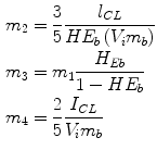
,  [min−1], instead, are rate parameters as follows:
 entering the bloodstream from the subcutaneous depots in the diabetic subject is described by a subcutaneous insulin infusion model (Fig. 6), whose model equations are:
(4)
 pmol/kg the amount of nonmonomeric and monomeric insulin in the subcutaneous space, respectively,
  [min−1] the rate constant of insulin dissociation,
  [min−1] and
  [min−1] the rate constants of nonmonomeric and monomeric insulin absorption, respectively, and
  [pmol/kg/min] the exogenous insulin infusion rate. The insulin flow
  which entered the bloodstream is degraded in the liver and the periphery according to the model equations [26]:
(5)
 [pmol/kg] and I l [pmol/kg] are insulin masses in plasma and liver, respectively,
  [L/kg] is the distribution volume of insulin, while
  [pmol/L] accounts for the total plasma insulin concentration.
  is the rate of hepatic clearance,
  ,
,  ,
,  [min−1], instead, are rate parameters as follows:
