Principles of Radiologic Physics and Dosimetry

James A. Purdy

A solid foundation in the principles of radiologic physics, dosimetry, and treatment planning is essential for the practice of modern-day radiation oncology. This chapter discusses the basic concepts in radiation physics, radiation therapy treatment machines, and the dosimetry parameters used for photon external beam treatment planning and dose/monitor unit calculations methods. As this textbook is aimed at practicing radiation oncologists and physician residents, these topics are not treated in the detail required for medical physicists. More details on these topics can be found in the medical physics textbooks listed in the references.^1–5

ATOMIC AND NUCLEAR STRUCTURE

The atom may be thought of as consisting of a centrally located core, the nucleus, surrounded by small orbiting particles called electrons. The overall dimension of an atom is about 10⁻¹⁰ m, and the nucleus is about 10⁻¹⁴ m. An electron has a rest mass (m_e) of 9.109 × 10⁻³¹ kg and has a negative electrical charge equal to 1.602 × 10⁻¹⁹ coulomb (C). Most of the mass of the atom is contained in the nucleus, making it extremely dense (10¹⁵ kg/m³). The nucleus is composed of two kinds of particles—protons and neutrons, known collectively as nucleons. A proton has a rest mass (m_p) of 1.673 × 10⁻²⁷ kg and has a positive electrical charge equal in magnitude to the charge of the electron (1.602 × 10⁻¹⁹ C). Collectively, the protons constitute the electrical charge of the nucleus. A neutron is slightly more massive than a proton (m_n = 1.675 × 10⁻²⁷ kg) and has no electrical charge.

Units used to describe atomic processes include the atomic mass unit (amu) for mass, nanometer (nm) for distance, electron volt (eV) for energy, and electronic charge (e) for electrical charge. The amu is defined as 1/12 the mass of the neutral carbon-12 atom. Thus, 1 amu = 1.660 × 10⁻²⁷ kg. In terms of amu, a proton’s rest mass is equal to 1.00727 amu, a neutron’s rest mass is equal to 1.00866 amu, and an electron’s rest mass is equal to 0.000548 amu. The electron volt (eV) is defined as the kinetic energy acquired by an electron accelerated through a potential difference (voltage) of 1 volt (V). One electron volt is equal to 1.6 × 10⁻¹⁹ joule (J) of energy. One writes 1,000 electron volts (keV) as 10³ eV, and 1 million electron volts (MeV) as 10⁶ eV. The nanometer is defined as equal to 10⁻⁹ m, and the electronic unit of charge is defined as equal to 1.602 × 10⁻¹⁹ C.

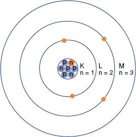
The planetary model of the atom is attributed to Niels Bohr, who in 1913 theorized that the hydrogen atom consisted of an electron orbiting around a nucleus of equal and opposite charge. He extended his theory to multielectron atoms, requiring the electrons surrounding a nucleus to be arranged in distinct, concentric shells or energy levels as shown in Figure 6.1. Energy is released when an electron moves to an orbit closer to the nucleus, and energy is required to move an electron into a higher orbit. Historically, the shells are labeled, from innermost outward, by the letters K, L, M, and so forth. There are a maximum number of electrons that can be accommodated in each shell: 2 in the first shell, 8 in the second, 18 in the third, and so on. The maximum number of electrons allowed in each shell is given by 2n², where n is an integer specific to each shell and is called the principal quantum number. Other properties of the electron also have discrete values specified by quantum numbers. These include the electron’s angular momentum as it orbits the nucleus, denoted by quantum number l (l = 0, 1,…, n – 1); its spin about its axis, denoted by s (s = ±1/2); and its magnetic moment, denoted by m_l (m_l = 0, ±1,…, ±l). Thus, each electron in an atom has an associated set of quantum numbers (n, l, s, m_l). This is the basis of the Pauli exclusion principle, which states that no two electrons can have the same set of quantum numbers within a particular atom.

Modern physics has replaced the simplistic orbiting electron model of Bohr with a complex quantum mechanical model of diffuse electron clouds that represent probability functions of the electron’s position. However, for an understanding of radiologic physics, the simple Bohr model of a nucleus composed of protons and neutrons and surrounded by orbiting electrons in distinct orbits (energy levels) is sufficient.

The atom of an element is specified by its atomic number, denoted by the symbol Z, and its mass number, denoted by the symbol A. The atomic number is equal to the number of protons in the nucleus, and the mass number is equal to the number of nucleons (protons and neutrons) in the nucleus. Hence, A minus Z is equal to the number of neutrons, denoted by the symbol N, within the nucleus. In addition, each element has an associated chemical symbol (e.g., Co for cobalt). When these definitions are used, the standard notation to specify an atom is , as illustrated by , which is a radioactive isotope of the element cobalt that has an atomic number of 27 (i.e., 27 protons) and a mass number of 60 (i.e., 60 nucleons, or 27 protons and 33 neutrons).

Isotopes of an element (e.g., , , and ) have the same atomic number but different numbers of neutrons and therefore different mass numbers. Isotopes have the same chemical properties but have different physical properties. Atoms such as and , which have the same mass number but different numbers of protons and neutrons, are called isobars. Atoms such as and , which have the same number of neutrons but different atomic and mass numbers, are called isotones.

FIGURE 6.1. Schematic drawing of the Bohr model of the atom. The nucleus contains protons (p) and neutrons (n). Electrons revolve around the nucleus in specific orbits having discrete energy levels. By convention, the orbits (energy levels) are assigned either quantum numbers (n = 1, 2, 3, …) or letters (K, L, M,…).

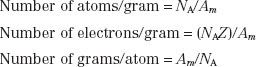
Every atom has a characteristic atomic mass A_m (sometimes referred to as atomic weight). The gram-atomic mass of an isotope is the amount of isotope in grams that is numerically equaled to the isotope’s atomic mass. For example, 1 g-atomic mass of carbon-12 is 12 g. One gram-atomic mass contains 6.0228 × 10²³ atoms, a constant that is called Avogadro’s number (N_A). Useful parameters that can be calculated using Avogadro’s number are as follows:

The closer the electrons are to the nucleus, the more tightly bound they are to the nucleus. This results from the attraction between the negatively charged electrons and the positively charged nucleus and is referred to as the Coulomb or electrostatic force. To move an electron from an inner shell to an outer shell (excitation) or to remove it completely from the atom (ionization), energy must be supplied. The energy required to remove an electron completely from an atom is called the binding energy for the electron. Binding energies are considered negative because energy must be supplied to remove the electron from its orbit. Atomic shells often are described in terms of binding energy, as shown in Figure 6.2 for the tungsten atom. The binding energies for the K, L, and M shells are –69,500, –11,000, and –2,500 eV, respectively. The electrons in the outermost shells are called valence electrons and have a binding energy of only a few electron volts because they are very loosely bound. These electrons determine the atom’s chemical properties.

FIGURE 6.2. Schematic drawing of tungsten atom showing electron configuration and energy levels. (From Johns HE, Cunningham JR. The physics of radiology, 4th ed. Springfield, IL: Charles C Thomas; 1983.)

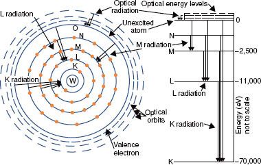
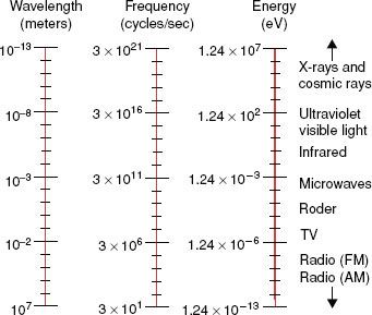
FIGURE 6.3. Electromagnetic spectrum extending over several orders of magnitude, with values of wavelength and frequency, and identifying values in some of the more common regions of the spectrum.

ELECTROMAGNETIC RADIATION

Electromagnetic radiation can be represented by a varying electric and magnetic field that is conveniently described using a sine-wave model. The sine wave is characterized by two parameters: the frequency, represented by the Greek letter v, and the wavelength, represented by the Greek letter λ. The wavelength is the distance from one crest of the sine wave to another; the frequency is the number of complete cycles or oscillations per second and is measured in hertz (Hz). The product of the frequency and wavelength is the speed with which the wave is propagated, which in a vacuum is the speed of light (c = 3 × 10⁸ m/sec).

Electromagnetic radiation wavelengths extend from approximately 10⁷ to 10⁻¹³ m. The frequencies associated with these radiations are approximately 10¹ to 10²¹ Hz. the electromagnetic spectrum shown in Figure 6.3 includes the radio and television bands; radar and microwaves; the infrared, visible, and ultraviolet regions; and x-rays and cosmic rays.

Quantum physics allows electromagnetic radiation to be represented as waves and also as particles, called photons. This is referred to as the wave–particle duality of nature. The photon energy is directly proportional to the classic wave frequency and is related to it through a constant of proportionality known as Planck’s constant (h), which has a numerical value of 6.625 × 10⁻³⁴ J-sec. The relationship between energy, E, and frequency, v, is given by the following equation:

The relationship between photon energy and photon wavelength is given by the following equation:

in which c is the speed of light in a vacuum. These relationships show that as the wavelength becomes shorter or the frequency becomes larger, the energy of the photon becomes greater.

X-RAYS

Wilhelm Conrad Röentgen discovered x-rays on November 8, 1895.⁶ He observed that a paper screen coated with fluorescent material glowed when placed in the vicinity of a tube of gas at low pressure through which electricity was being passed. We now know that the x-rays were produced where the electron beam struck the anode. Energetic electrons that impinge on matter interact with either the orbital electrons or the nuclei of target atoms. The kinetic energy of the electrons then is converted into thermal energy or electromagnetic energy (in the form of x-rays).

The impinging electron’s kinetic energy is converted into thermal energy through interaction with an outer-shell electron of a target atom, which raises it to a higher energy level (referred to as excitation). The excited electron then returns to the normal energy level with the emission of low-energy electromagnetic radiation (infrared).

If the impinging electron’s kinetic energy is high enough, the interaction can free an orbital electron (referred to as ionization), which then can result in the production of electromagnetic radiation (characteristic x-rays) when an outer orbital electron moves to the electron vacancy produced via ionization (Fig. 6.4). The characteristic x-ray energy is equal to the difference in the binding energies of the two orbital electrons involved. Occasionally, this excess energy is transferred directly to another orbital electron, causing it to be emitted from the atom. Such electrons are called Auger electrons.

The impinging electron also can lose its kinetic energy via a process called bremsstrahlung (braking radiation), which occurs when the incident electron interacts with the electric field of the nucleus (rather than the orbiting electrons) and is deflected and loses energy. This loss of energy reappears in the form of an x-ray photon. The impinging electron can lose any amount of its kinetic energy in the bremsstrahlung process. Thus, the x-radiation produced via the bremsstrahlung process is characterized by having a continuous range of energy values, unlike characteristic x-rays, which have only discrete energy values. A bremsstrahlung spectrum (i.e., a graph of x-ray intensity vs. energy) is shown in Figure 6.5. Superimposed on the continuous bremsstrahlung x-ray spectrum are the characteristic x-rays. The maximum energy of a bremsstrahlung x-ray is numerically equal to the maximum energy of the incident electrons. The direction of emission of the bremsstrahlung x-ray depends on the energy of the incident electron, with higher-energy electrons producing more-forward-directed x-rays.

FIGURE 6.4. Schematic diagram illustrating characteristic x-ray production.

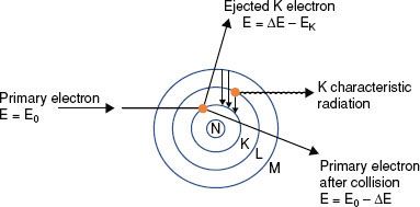
FIGURE 6.5. A bremsstrahlung x-ray spectrum calculated for a thick tungsten target extending from zero to the maximum energy of the electron. The dotted lines are for no filtration, and the solid curves are for a filtration of 1-mm aluminum. Note the superimposed characteristic x-ray emission spectrum. (From Johns HE, Cunningham JR. The physics of radiology, 4th ed. Springfield, IL: Charles C Thomas; 1983.)

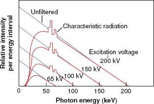
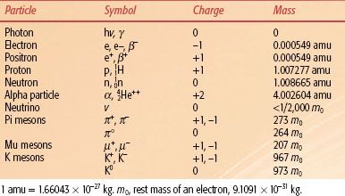
TABLE 6.1 PARTICLES OF INTEREST IN RADIATION THERAPY

RADIOACTIVITY

In 1896 Henri Becquerel conducted experiments in which he wrapped a photographic plate in black paper to keep out the light and then placed pieces of various elements against the wrapped plate.⁷ He discovered that the mineral pitchblende emitted x-rays. Other elements—such as thorium, actinium, and two new elements (polonium and radium) discovered by Pierre and Marie Curie⁸—also emitted x-rays. Further experiments showed that the radioactive elements emitted three types of radiation: α-particles, having a positive electrical charge; β-particles, having a negative charge; and high-energy γ-rays, having no charge at all. We now know that an α-particle is a helium nucleus, β-particles are electrons, and γ-rays are electromagnetic radiation that is similar to x-rays except that it originates from within the nucleus of the atom.

Many other elementary particles have since been discovered and are important topics of current physics research, but they are not germane to our discussion of radiation oncology physics. Properties of the particles relevant to radiation therapy are listed in Table 6.1.

The radioactive decay processes are related to the forces involved. Huge electrostatic (Coulomb) forces of repulsion exist between the positively charged and closely spaced protons in a nucleus. However, a nuclear force of attraction (called the strong nuclear force) exists among the neutrons and protons, binding them together to form the nucleus. The strong nuclear force is much more complicated than the electrostatic (Coulomb) force and is still not completely understood. However, it is known that the strong nuclear force between nucleons depends on the distance between them and is effective only over a very short distance, whereas the electrostatic force decreases with the square of the distance. The strong nuclear force easily overcomes the repelling electrostatic force as long as the protons are very close together. However, for a large nucleus, the strong nuclear force binding the nucleons together may be weaker on opposite sides of the nucleus than the repelling electrostatic force. Therefore, a large nucleus is not as stable as a smaller nucleus.

Because neutrons interact through the attractive strong nuclear force and not the repelling electrostatic force, they can be considered stabilizing particles for the nucleus. For example, in light nuclei, only an equal number of neutrons and protons are required, but in heavier nuclei, the number of neutrons must be about 1.5 times greater than the number of protons to counteract the repelling electrostatic forces of the protons. A nuclide having too many more protons than neutrons is said to have an unfavorable N-to-Z ratio and thus undergoes radioactive decay to reach a stable configuration.

The decay constant of a radioactive nucleus is defined as the fraction of the total number of atoms that decay per unit of time and is denoted by the symbol λ. The decay process can be represented mathematically. If N₀ radioactive nuclei are initially present in a particular sample, the number of radioactive nuclei, N, remaining at a particular time, t, is given by the following equation:

Activity, which describes the radioactivity of a sample and is denoted by the symbol A, is defined as the total number of disintegrations per unit of time interval and is given by the following relationship:

This decay-constant equation can be expressed in terms of activity:

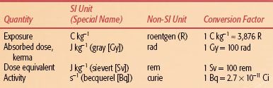
where A is the activity at time t and A₀ is the initial activity. The curie (Ci), a unit of activity, is equal to 3.7 × 10¹⁰ disintegrations per second, the approximate number of decays per second by 1 g of ²²⁶Ra. The becquerel (Bq), the special name in the International System of Units (SI) for the measure of activity, is equal to one disintegration per second (Table 6.2).

The half-life of a radioactive nuclide is the time required for the number of atoms in a particular sample to decrease by one-half. The half-life, T_1/2, is related to the decay constant by the following equation:

The average life, T_a, of a radioactive nuclide is related to the decay constant and the half-life by the following equation:

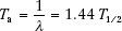
The average life represents the time period that a hypothetical source would need—if it retained its original activity for that time period and then suddenly decayed to zero activity—to produce the same number of disintegrations as produced over an infinite time period by the source if it decayed exponentially.

Gamma decay occurs when a nucleus undergoes a transition from a higher to a lower energy level. In this process, a high-energy photon, called a γ-ray, is emitted. These γ-rays are identical to the x-rays emitted by excited atoms, except that γ-rays originate from within the nucleus and x-rays originate from outside the nucleus. Half-lives for γ decay are usually very short, typically 10⁻¹⁵ second.

Closely related to γ decay is the process called internal conversion. Instead of emitting a γ-ray, the excess energy from the excited nucleus is transferred to an electron in one of the inner atomic shells, causing ejection of the electron from the atom with emission of characteristic x-rays. The probability of internal conversion occurring increases as the atomic number increases.

In β decay, a neutron within the nucleus is converted into a proton, and an electron and an antineutrino are emitted, or a proton is converted into a neutron, and a positron and a neutrino are emitted:

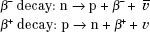
TABLE 6.2 INTERNATIONAL SYSTEM OF UNITS (SI UNITS) FOR RADIATION THERAPY

The positron was discovered in cosmic ray experiments in 1932. It is a positively charged particle with the same mass and spin as the electron and is considered the antiparticle of the electron. The neutrino and its antiparticle, the antineutrino, are massless particles (or at least have a very small mass) having no charge that carry opposite spins and account for the conservation of energy and continuous energy spectrum observed for β decay. Particle–antiparticle pairs interact by annihilating each other, converting all their mass into electromagnetic energy (two γ-ray photons, each of 0.51 MeV). In β decay, the emitted particles may vary in the kinetic energy they possess, which is rarely > 3MeV. Half-lives for β decay are long compared with γ decay half-lives, varying from seconds to years. The forces responsible for the β decay processes are weak compared with both the strong nuclear force and the electrostatic force among the nucleons. Accordingly, the force responsible for β decay is referred to as the weak nuclear force.

Electron capture is an alternative to positron decay. In this process, an electron, usually in the K shell, is captured within the nucleus and combined with a proton to create a neutron. Electron capture most often is followed by γ decay to release any excess nuclear energy.

Alpha decay occurs in nuclides with atomic number >82 and where the ratio of neutrons to protons is low, thus resulting in the repulsive Coulomb force of the protons overcoming the attractive strong nuclear force. The emitted α-particle is a helium nucleus (two protons and two neutrons). The kinetic energy for a particular α decay is monoenergetic (i.e., the transition may be to an excited energy state with subsequent γ emission) and often 4 to 5 MeV. Half-lives range from 10⁻³ to 10¹⁰ years. The radioactive decay of radium to radon is an example of α decay, where the Q term represents the total energy release in the transition (called transition energy). For example,

The most recent version of the periodic table of the elements shows a grouping of 118 elements (elements 117 and 118 have not yet been observed but are included to show their expected positions). Only the first 92 occur naturally; the remaining ones have been produced artificially. In general, the elements with high atomic number tend to be radioactive; in fact, all but one of the elements with atomic number >82 (lead) are radioactive; only Bi is stable.

The naturally occurring radioactive elements have been grouped into three radioactive series called the uranium series, the actinium series, and the thorium series, all of which terminate with a stable isotope of lead. The uranium series provides an example of radioactive nuclides undergoing successive transformations through α and β decay in which the parent nuclide produces a radioactive product called the daughter nuclide.

When the half-life of the parent nuclide is longer than the half-life of the daughter nuclide, an equilibrium condition exists. When this occurs, the ratio of the activity of the daughter nuclide to the activity of the parent nuclide becomes constant, and the apparent decay rate of the daughter nuclide is controlled by the parent nuclide’s decay rate. Two types of radioactive equilibrium conditions are defined: transient equilibrium and secular equilibrium. Transient equilibrium is established when the parent nuclide’s half-life is not much greater than the daughter nuclide’s half-life (Fig. 6.6). In secular equilibrium, the half-life of the parent nuclide is much greater than that of the daughter nuclide (Fig. 6.7). The two types of equilibrium are described mathematically by the following equations, in which A_P and A_D represent the activity of the parent and daughter nuclides, respectively:

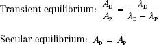
FIGURE 6.6. Transient equilibrium. Shown is a semilog plot of activity versus time for parent and daughter radionuclides illustrating conditions of transient equilibrium that may be achieved when the parent nuclide’s half-life is not much greater than the half-life of the daughter nuclide. Once equilibrium is established, the daughter activity exceeds the parent activity, and both decay with the half-life of the parent.

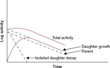
FIGURE 6.7. Secular equilibrium. Shown is a semilog plot of activity versus time for parent and daughter radionuclides illustrating conditions of secular equilibrium that may be achieved when the parent nuclide’s half-life is much greater than the half-life of the daughter nuclide. Once secular equilibrium is established, activities of both parent and daughter are equal.

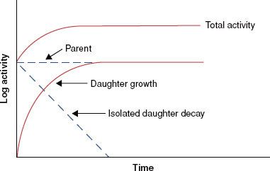
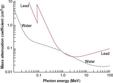
FIGURE 6.8. Mass attenuation coefficient for lead and water. Note sharp discontinuities, which are called absorption edges. (From Johns HE, Cunningham JR. The physics of radiology, 4th ed. Springfield, IL: Charles C Thomas; 1983.)

INTERACTION OF PHOTONS WITH MATTER

As stated previously, x-rays and γ-rays may be considered as bundles of energy called photons. If an x-ray photon enters a thin layer of matter, it is possible that it will pass through without interaction, or it may interact (usually with the atomic electrons, but sometimes with the atomic nuclei) in one of five different ways (coherent scattering, photoelectric effect, Compton scattering, pair production, and photodisentegration). The probability that a photon will interact when it traverses through a given thickness of material is the product of the individual interaction probabilities for each of these processes. The attenuation process can be described mathematically by the following equation:

where N₀ is the number of photons in the beam impinging on an absorber of thickness x, e is the base of the natural logarithms, and μ is the linear attenuation coefficient. The quantity μ is actually the sum of the individual attenuation coefficients for the five processes. Its numerical value depends on the energy of the photon and the type of attenuating material.

There are a variety of tabulated attenuation coefficients, including the linear attenuation coefficient (μ), the mass attenuation coefficient (μ/ρ), the mass energy-transfer coefficient (μ_t/ρ), and the mass energy-absorption coefficient (μ_en/ρ). Each type of coefficient is intended for use in the solution of different types of attenuation or energy-absorption problems; division by ρ, the physical density of the medium, makes the coefficient medium independent. Figure 6.8 shows the mass attenuation coefficient for lead and water as a function of incident photon energy. The discontinuities where the attenuation coefficient suddenly increases are called absorption edges and occur at photon energies just equal to the binding energy of a specific electron shell.

The thickness of material that reduces the number of photons transmitted to one-half the incident number is termed the half-value layer (HVL). The HVL is related to the linear attenuation coefficient by the following equation:

This parameter is used to describe the quality or penetrability of the radiation and is discussed later in this chapter.

Coherent or Classical Scattering

If the photon energy is low enough that the quantum effects of the interaction are unimportant and the bound electron(s) can be regarded as essentially “free,” the interaction corresponds to the “classical scattering” situation (called coherent scattering), in which the incident electrical field accelerates one or more orbital electrons and causes them to radiate. There are two types of coherent scattering: Thomson scattering, in which a single orbital electron is involved, and Rayleigh scattering, in which the orbital electrons act as a single group. In coherent scattering, no energy is transferred; only the direction of the incident photon is changed. The coherent mass attenuation coefficient is denoted by σ_coh/ρ.

FIGURE 6.9. Photoelectric effect. In this type of photon interaction, the incident photon disappears, and an electron is ejected with kinetic energy equal to the incident photon’s energy minus the binding energy of the electron. Characteristic x-rays and Auger electrons are emitted as the atom’s electrons cascade to fill the vacancy created by the ejected electron.

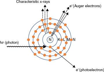
FIGURE 6.10. Compton effect. In this type of photon interaction, the incident photon interacts with one of the atom’s outer electrons, and the energy is shared between the ejected electron and a scattered photon.

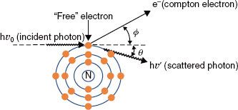
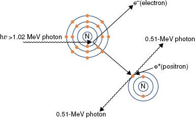
FIGURE 6.11. Pair production. In this type of photon interaction, the incident photon interacts with the electromagnetic field of the nucleus. The incident photon disappears, and two energetic electrons (a positron and a negatron) are produced. Two annihilation photons of energy 0.511 MeV then are produced when the positron interacts with its antiparticle, another electron.

Photoelectric Effect

In the photoelectric effect, the total energy of the photon is transferred to an orbital electron, usually close to the nucleus, and the photon disappears. The electron then is ejected from the atom with an energy equal to the energy of the photon minus the binding energy of the electron (Fig. 6.9). The direction in which the electron is emitted depends on the energy of the incident photon. For the low-energy photons (e.g., 50 keV) the photoelectron is ejected at a large angle with respect to the incoming photon’s direction, increasing in the forward direction as the photon’s energy increases. After ejection of the electron, the neutral atom becomes a positively charged ion with a vacancy in an inner shell that must be filled. The atom returns to a stable condition by filling the vacancy with a nearby, less tightly bound electron farther out from the nucleus, and characteristic x-rays or an Auger electron is emitted.

The probability that a given photon will interact by means of the photoelectric process (denoted by τ/ρ) is a function of both the photon’s energy and the atomic number of the target atom. For the process to occur, the incident photon must have energy greater than the binding energy of the involved orbital electron. In general, the probability per electron that a photon will undergo a photoelectric interaction is inversely proportional to the third power of the photon’s energy and directly proportional to the third power of the atomic number of the target atom.

Compton Scattering

In Compton scattering, the incident photon interacts with a loosely bound orbital electron in which part of the photon’s energy is transferred to the electron as kinetic energy and the remaining energy is carried away by another photon (Fig. 6.10). The binding energy of the electron is insignificant compared with the incident photon’s energy and thus can be ignored. The energy of the Compton-scattered photon is equal to the difference between the energy of the incident photon and the energy transferred to the electron. If the incoming photon’s energy is low (e.g., 100 keV), very little energy is transferred to the electron. As the photon’s energy increases, a greater proportion of the energy is transferred to the electron, so the scattered photon necessarily retains a smaller proportion of the incident energy. The photon may be scattered at any angle with respect to the direction of the incident photon, but the Compton electron is confined to angles between 0 and 90 deg with respect to the direction of the incident photon. If the incoming photon’s energy is low, the distribution of the scattered photons is isotropic (equal in all directions). The scatter angles decrease for photons and electrons as the incident photon’s energy increases (e.g., at megavoltage photon energies, both are scattered predominantly in the forward direction).

As a result of conservation of energy and momentum, the energies of the incident photon, hv₀, the scattered photon, hv′, and the scattered electron, E, are given by the following relationships:

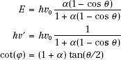
where α = hv₀/m₀c², and m₀c² is the rest energy of the electron (0.511 MeV). If hv₀ is expressed in MeV, then α = hv₀/0.511.

The probability that a photon will interact with a target atom via the Compton process (σ_c/ρ) depends on the energy of the incoming photon, generally decreasing as the energy of the photon is increased. The probability of a Compton interaction is nearly independent of the atomic number of the absorber and is directly proportional to the number of electrons per gram.

Pair Production

Pair production (Fig. 6.11) is possible only with photons having energies >1.02 MeV. When such an energetic photon approaches closely enough to the nucleus of the target atom, the incident photon energy may be converted directly into an electron–positron pair. Energy possessed by the photon in excess of 1.02 MeV appears as kinetic energy, which may be distributed in any proportion between the electron and the positron. When the positron comes to rest, it combines with an electron, and both particles then undergo mutual annihilation, with the appearance of two photons with energy of 0.511 MeV traveling in opposite directions. The probability of pair production (π/ρ) occurring increases rapidly with incident photon energy above the 1.02-MeV threshold and is proportional to Z² per atom, Z per electron, and approximately Z per gram.

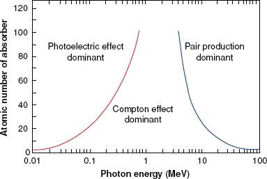
FIGURE 6.12. Relative importance of the three principal modes of interaction as a function of photon energy and atomic number of absorber. (From Hendee WR, Ritenour ER. Medical imaging physics, 3rd ed. St. Louis: Mosby-Year Book; 1992.)

Photodisintegration

In photodisintegration, a high-energy photon interacts with the nucleus of an atom, totally disrupting the nucleus, with the emission of one or more nucleons. It typically occurs at photon energies much higher than those encountered in radiation therapy. However, it is important to account for this in designing shielding around high-energy accelerators, as this interaction is a source of low-energy neutrons.

Relative Importance of Interaction Processes

Figure 6.12 illustrates the relative importance of the photoelectric, Compton, and pair-production processes—the three principal modes of interactions pertinent to radiation therapy—as a function of energy and atomic number of the absorber. For example, for an absorber with an atomic number approximately equal to that of tissue (Z = 7) and for monoenergetic photons, the photoelectric effect is the dominant interaction below about 30 keV. Above 30 keV, the Compton effect becomes dominant and remains so until approximately 24 MeV, at which point pair production becomes the dominant interaction. The total mass attenuation coefficient accounting for all the photon interactions discussed is given by the sum of the individual coefficients:

INTERACTION OF PARTICLES WITH MATTER

Electrons

An electron loses its kinetic energy when traversing matter via interactions that can be either elastic, in which no kinetic energy is lost, or inelastic, in which some portion of the kinetic energy is changed into some other form of energy. Elastic collisions occur with either atomic electrons or with atomic nuclei and are characterized by a change in direction of the incident electron with no loss of kinetic energy. Inelastic collisions can occur with atomic electrons, resulting in ionizations and excitations of atoms, or inelastic collisions with atomic nuclei, which result in the production of bremsstrahlung x-rays (radiative losses). In the case of ionization, it is possible for the ejected electron to acquire enough kinetic energy to cause additional ionizations of its own. These electrons are called secondary electrons or δ rays, and they can go on to produce additional ionizations and excitations. The typical energy loss in tissue for a therapeutic electron beam, averaged over its entire range, is about 2 MeV/cm in water.

The complete description of the energy and depth of penetration of the moving electrons at any point in the medium is complicated by the fact that the electrons are very much lighter than the atomic nuclei. As a result, the electron can lose a very large fraction of its energy in a single process and thus can be deflected by very large angles. This means that even if the electron beam is monoenergetic when first impinging on a medium, there will be a large variation among all the moving electrons as to where in the medium each will stop. This is referred to as range straggling.

Protons and Light Ions

Protons traverse relatively straight paths through matter, slowing down continuously by interactions with atomic electrons and with atomic nuclei. This results in depth–dose characteristics that show an approximately constant absorbed dose value over most of the beam range until near the end of the proton’s range, where a very sharp increase in dose occurs (called the Bragg peak), as shown in Figure 6.13. Dose at the peak is approximately four times the dose at the surface, and the distal width of the peak is on the order of 1 cm, depending on beam energy and beam energy spread. Depth–dose characteristics customized for individual patients can be generated by superposition of multiple proton beams having different energies. This technique creates a spread-out Bragg peak that covers the target volume and decreases sharply to zero dose a few millimeters beyond the target. The relative biologic effectiveness (RBE) of proton beams is similar to that of other low-linear-energy transfer radiation, such as photon and electron beams. Pagnetti et al.⁹ measured RBE equal to 1.0 in the plateau region and 1.1 in the center of the Bragg peak for a 250-MeV beam. Therefore, the clinical response established for photon and electron treatments is considered applicable to proton treatments.

Neutrons

Neutrons, like photons, are uncharged and thus are an indirectly ionizing radiation, which are exponentially attenuated by matter. The interactions are through processes that are primarily nuclear. They include elastic scattering with nuclei that make up the body’s tissues (hydrogen, oxygen, carbon, nitrogen, etc.). Neutron interactions result in recoil protons and charged nuclear fragments that have relatively low energy. The RBEs of these resultant particles are not fully known, thereby complicating the understanding of the relationship between clinical response and absorbed dose.

RADIATION THERAPY TREATMENT MACHINES

Kilovoltage Units

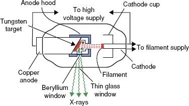
Before 1951, most radiation treatment units were kilovoltage x-ray machines capable of producing photon beams having only limited penetrability. Today, this type of machine is still used in some clinics for the treatment of skin cancer. In these machines, the electrons are accelerated by an electric field produced from a high voltage generated in a transformer that is applied directly between the filament (cathode) and the x-ray target (anode). A schematic diagram of a radiation therapy x-ray tube is shown in Figure 6.14. The potential difference (kVp) is variable on these machines, and metal filters can be added to absorb the lower-energy photons preferentially, changing the penetrability of the beam. The combination of variable kVp and different filtration provides the capability of generating multiple x-ray beams. The degree of penetrability is used to categorize the units as contact, superficial, and orthovoltage (deep-therapy) x-ray machines. A more detailed review of these type of treatment machine is provided by Biggs et al.¹⁰

FIGURE 6.13. Drawing illustrating the way in which the Bragg peak for a proton beam can be spread out. Curve A is the depth–dose distribution for the primary beam of 160-MeV protons at the Harvard cyclotron. Beams of lower intensity and shorter range, as illustrated by curves B to E, can be added to give a composite curve, S, which results in a uniform dose of >2.8 cm. (From Hall EJ. Radiobiology for the radiologist, 4th ed. Philadelphia: JB Lippincott; 1994.)

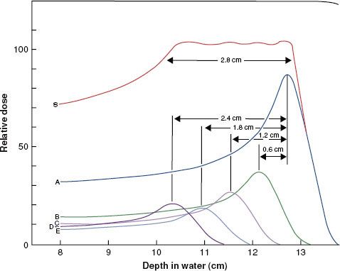
FIGURE 6.14. Schematic diagram of radiation therapy x-ray tube. (From Khan FM. The physics of radiation therapy, 3rd ed. Baltimore: Williams & Wilkins; 1994.)

Contact Units

A contact x-ray machine typically operates at potentials of 40 to 50 kVp and at a tube current of 2 to 5 milliamperes (mA). Attached cones are used for a source–skin distance (SSD) of typically 2 cm or less. Filters of 0.5- to 1.0-mm aluminum are used to give a typical HVL of 0.6-mm aluminum. The x-ray tube is rod shaped with an extremely thin mica–beryllium window, having an inherent filtration of 0.03-mm-aluminum equivalence, and the radiation is emitted axially. The primary radiation therapy application of a contact x-ray unit is for endocavitary irradiation of selected small rectal carcinomas.^11,12

Superficial Units

A superficial unit is an x-ray machine that operates at potentials of 50 to 150 kVp and 5 to 10 mA. Added thickness of filtration (1-mm Al to 1-mm Al + 0.25-mm Cu) produces HVLs of 1.0 to 8.0 mm of aluminum. Attached cones typically are used; lead masks are used to define irregular fields. The SSD is typically 15 or 20 cm. These machines are used primarily to treat skin lesions.

Orthovoltage (Deep-Therapy) Units

Orthovoltage x-ray machines operate at potentials between 150 and 500 kV, with most operating between 200 and 300 kV, and with tube currents of 10 to 20 mA. HVLs of 1 to 4 mm of copper are common with the use of added filters, such as the Thoraeus filter, a combination of thin sheets of tin, copper, and aluminum arranged so that the highest–atomic number sheet is always closest to the x-ray target, ensuring that the higher-energy characteristic x-rays are absorbed by the lower-Z metal. Treatment fields usually are defined using detachable cones. The SSD is typically 50 cm. Very few of these types of machines are still in clinical use.

Supervoltage and Megavoltage Photon and Electron Beam Treatment Units

X-ray treatment machines operated in the range of 500 to 1,000 kV were designated as supervoltage therapy machines.¹³ The resonant transformer x-ray machine is an example of this type of kilovoltage machine. X-ray treatment machines that can produce beams 1 MV or greater have been designated as megavoltage therapy machines. One of the first megavoltage machines was the Van de Graaff generator, which operated at 1 to 2 MV. Another early type of megavoltage machine was the betatron, first developed in 1941 by Kerst.¹⁴ Betatrons used in radiation oncology produced x-ray beams with energies of >40 MV. All of these early machines are now obsolete and no longer in clinical use. Details on the history and development of these early accelerators used in radiation therapy can be found in the textbook by Karzmark et al.¹⁵

Cobalt-60 Teletherapy

The first cobalt-60 (⁶⁰Co) teletherapy machine was loaded with its ⁶⁰Co source in August 1951 in the Saskatoon Cancer Clinic, Saskatoon, Canada, and the first patient was treated on November 8 of that year.^16,17 A detailed review of ⁶⁰Co teletherapy machines is provided by Glasgow.¹⁸ The advantages of a ⁶⁰Co teletherapy machine are its relative constancy of beam output, predictability of decay because of a well-defined half-life, and lack of day-to-day small-output fluctuations typically found in electrical machines. Disadvantages include the need for source replacement approximately every 4 to 5 years, poor field flatness for large fields and large penumbra, and lower depth dose compared with high-energy photons generated by medical linear accelerators and discussed later. These types of machines became a mainstay for radiation therapy for nearly three decades but are rarely used in U.S. clinics today. Isocentric units with source-to-axis distance (SAD) of 80 or 100 cm were designed with maximum field sizes of 40 × 40 cm at the machine isocenter for the 100-cm SAD machine. Source activities vary from about 5,000 to 13,000 Ci in 1.5- to 2.0-cm-diameter sources and yield exposure rates from 150 to 250 R/min at 1 m. The radiation consists of 1.17- and 1.33-MeV γ-rays having a d_1/2 in tissue (the depth at which the dose has been reduced to 50% of the maximum dose value) of about 10 cm.

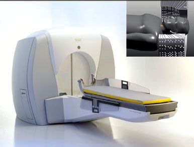
FIGURE 6.15. Elekta Gamma Knife (Elekta AB, Stockholm, Sweden) is a dedicated stereotactic radiosurgical device first developed in 1968 by Dr. Lars Leksell, a Swedish neurosurgeon, to provide highly accurate radiation ablative treatment of intracranial targets. Shown is the latest model, the Gamma Knife Perfexion, which broadens both the techniques and the scope of treatments, including the ability to treat lesions in the upper cervical spine.