Photon External-Beam Dosimetry and Treatment Planning

James A. Purdy and Eric E. Klein

The radiation oncologist, when planning the treatment of a patient with cancer, is faced with the problem of prescribing a treatment regimen with a radiation dose that is large enough potentially to cure or control the disease, but does not cause serious normal tissue complications. This task is a difficult one because tumor control and normal tissue effect responses for most disease sites are typically steep functions of radiation dose; that is, a small change in the dose delivered (±5%) can result in a dramatic change in the local response of the tissue (±20%).^1,2,3 Moreover, the prescribed curative doses are often, by necessity, very close to the doses tolerated by the normal tissues. Thus, for optimum treatment, the radiation dose must be planned and delivered with a high degree of precision.

One can readily compute the dose distribution resulting from photons, electrons, protons, or a mixture of these radiation beams impinging on a regularly shaped, flat-surface, homogeneous unit-density phantom. However, the patient presents a much more complicated situation because of irregularly shaped topography and having tissues of varying densities and atomic composition (called heterogeneities). In addition, beam modifiers, such as wedges, compensating filters, or bolus, are sometimes inserted into the radiation beam, further complicating the calculation of the absorbed dose.

In this chapter, several aspects of photon external-beam treatment planning and dosimetry are reviewed, including methods used for dose/monitor unit calculations, correction for the effects of the patient’s irregular surface and internal heterogeneities on the calculated photon dose distribution, isodose distributions for combined fields, field junctions, field shaping and design of treatment aids, and related clinical dosimetry issues.

DOSE CALCULATION METHODS

For purposes of discussion, it is convenient to characterize photon beam dose calculation methods as either correction based or model based.⁴ In the former method, the dose at a given point is calculated using measured central-axis data, for example, percent depth dose (PDD), tissue-air ratios (TARs), tissue-maximum ratios (TMRs), tissue-phantom ratios (TPRs), and off-axis ratios (OARs). These quantities are measured under reference conditions (i.e., in a homogeneous water phantom with a flat surface normal to the incident radiation beam at a standard distance from the x-ray source). Hence, specific correction factors (CFs) are used in planning the treatment of real patients to account for varying patient surfaces, tissue heterogeneities, irregular field shapes, and any beam modifiers used.

In the model-based algorithms, the dose distribution is computed in a phantom or patient from more of a first-principles approach accounting for lateral transport of radiation, beam energy, geometry, beam modifiers, patient surface topography, and electron density distribution, rather than correcting parameterized dose distributions measured in a water phantom. These models utilize convolution energy deposition kernels that describe the distribution of dose about a single primary photon interaction site, and provide much more accurate results even for complex heterogeneous geometries. Both methods are discussed in the following sections and more details on model-based photon dose calculation algorithms can be found in the references listed.^4,5

Correction-Based Dose Calculation Methods

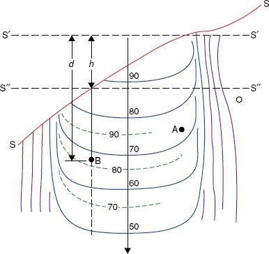
Using the notation of Khan et al.,⁶ the dose at a point (D_P) at a depth d of overlying tissue on the central ray for an irregularly shaped field is given by:

where S_c denotes the collimator scatter factor, Sp the phantom scatter factor, and TMR the tissue-maximum ratio. TF and WF denote the tray and wedge factors, respectively, and are defined as the ratio of the central ray dose with the tray or wedge filter in place relative to the dose in the open-beam geometry. The collimated field size is denoted by r_c and is usually described as the square field size equivalent to the rectangular collimator opening projected to isocenter. The effective field size is denoted by r_d and is specified to the isocenter distance (SAD). The inverse-square law factor accounts for the difference in distances from the source-to-point of dose calculation relative to the source to calibration point distance (SCD). Note that when isocentric calibration is used, this factor is unity. Also, note that collimator-defined field size is used for lookup of the collimator scatter factor, S_c, whereas effective field size projected to isocenter is used for lookup of the TMR value and the phantom scatter factor, Sp. By separately accounting for the effect of collimator opening on the primary dose component and the influence of cross-sectional area of tissue irradiated, most of the difficulties in accurately calculating a dose in the presence of extensive blocking are overcome. Details on determining the effective field size for an irregularly shaped field, taking into account both the primary and scatter dose components, will be discussed in a later section.

Correction for Varying Patient Topography (Air Gaps)

In the previous equation, it is assumed that the beam is normally incident on a unit-density uniform phantom. The following CF methods can be applied to the equation to account for the nonnormal beam incidence caused by the patient’s varying surface.⁷

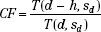
FIGURE 7.1. Schematic drawing illustrating tissue-air ratio and effective source-to-skin distance (SSD) methods for the correction of isodose curves under a sloping surface (solid lines for SSD = S′′; dashed lines for SSD = S′′). (From International Commission of Radiation Units and Measurements. Report 24: Determination of absorbed dose in a patient irradiated by beams of × or gamma rays in radiotherapy procedures. Washington, DC: International Commission of Radiation Units and Measurements, 1976.)

Air Gap CF: Ratio of Tissue-Air Ratio Method

In the ratio of TAR or TPR method, the surface (along a ray line) directly above point A (source-to-skin distance [SSD] = S′) is unaltered, so the primary component to the dose distribution at this point is unchanged (and the scatter component is also assumed to be unaltered) (see Fig. 7.1). Thus, the dose at point A can be considered as unaltered by patient shape. However, for point B, where there are considerable variations in the patient’s topography, both the primary and scatter components of the radiation beam are altered. The CF may be determined using two TARs or TPRs as follows:

where h = air gap.

Air Gap CF: Effective Source-Skin Ratio Method

In the effective SSD method, the isodose chart to be used is placed on the patient’s contour representation, positioning the central axis at the distance for which the curve was measured (Fig. 7.1). It then is shifted down along the ray line for the length of the air gap, h, resulting in SSD = S″. The PDD value at point B is read and modified by an inverse-square calculation to account for the effective change in the peak dose. The CF can be expressed as follows:

Correction for Tissue Heterogeneities

The following CF methods can be used to account for the tissue heterogeneities found within the patient.

Tissue Heterogeneities CF: Ratio of Tissue-Air Ratio Method

The ratio of TAR (RTAR) method of correction for inhomogeneities is given by:

where the numerator is the TAR for the equivalent water thickness, d_eff, and the denominator is the TAR for the actual thickness, d, of tissue between the point of calculation and the surface along a ray passing through the point. S_d is the dimension of the beam cross-section at the depth of calculation. The RTAR method accounts for the field size and depth of calculation. It does not account for the position of the point of calculation with respect to the heterogeneity. It also does not take into account the shape of the inhomogeneity; instead, it assumes that it extends the full width of the beam and has a constant thickness (i.e., referred to as slab geometry).

Tissue Heterogeneities CF: Power Law TAR Method

The power law TAR method was proposed by Batho⁸ and generalized by Young and Gaylord.⁹ This method, sometimes called the Batho method, attempts to account for the nature of the inhomogeneity and its position relative to the point of calculation. However, it does not account for the extent or shape of the inhomogeneity. The correction factor for the point P is given by:

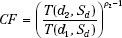
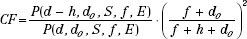
where d₁ and d₂ refer to the distances from point P to the near and far side of the non–water-equivalent material, respectively; S_d is the beam dimension at the depth of P; and ρ₂ is the relative electron density of the inhomogeneity with respect to water.

Sontag and Cunningham¹⁰ derived a more general form of this correction factor, which can be applied to a case in which the effective atomic number of the inhomogeneity is different from that of water and the point of interest lies within the inhomogeneity. The correction factor in this situation is given by:

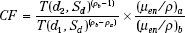
where ρ_a is the density of the material in which point P lies at a depth d below the surface and ρ_b is the density of an overlying material of thickness (d₂ – d₁); (μ_en/ρ)_a and (μ_en/ρ)_b are the mass energy absorption coefficients for the medium a and b.

Model-Based Dose Calculation Methods

Advanced three-dimensional dose calculation algorithms, such as the convolution/superposition algorithm and Monte Carlo, should now be considered the standard of practice.^4,5,11–13 These models provide accurate results even for complex heterogeneous geometries.

Convolution/Superposition Dose Calculation Algorithm

The convolution/superposition dose calculation algorithm is based on the following equation⁴:

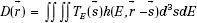
where D represents the dose at some point , T_E() represents the total energy released by primary photon interactions per unit mass (or TERMA), and h(E, – ) is the point-spread function (also called dose spread array, differential pencil beam, and energy deposition kernal). The point-spread function represents the fraction of the energy deposited (per unit volume) at point that is subsequently transported to the calculation point, . Hence, the dose at point is computed by integrating over all space the contributions from photons and electrons produced at all other points in the phantom or patient.

Ahnesjö et al.¹⁴ showed that the point-spread function, h(E, – ), changes only slightly as a function of energy, and thus, can be replaced by h( – ) (defined as the average point-spread function weighted by the spectral components of the beam), reducing the basic convolution four-dimensional integral to a three-dimensional integral over all space. Point-spread functions for monoenergetic photons are generally precomputed using Monte Carlo methods.¹⁴ The energy dependence of the TERMA, T_E (), can be expressed by applying the inverse-square law and exponential attenuation to the photon fluence at the surface of the phantom or patient.

The three-dimensional integral is typically evaluated in a two-step process. The first step takes into account the properties of the accelerator (including the finite source size, primary collimator, flattening filter, collimator jaws, multileaf collimators, and any beam-modifying devices used for the treatment, such as wedges, alloy blocks, and compensating filters) to compute the energy fluence at the phantom or patient surface. The second step of the calculation takes into account the inverse-square law and exponential attenuation to this incident fluence to determine the TERMA, T_E(), at each point within the phantom or patient and convolve the result with the point-spread function, h(–).

The convolution equation is strictly valid only for homogeneous media (i.e., h() must be spatially invariant). To account for the effects of tissue heterogeneities, all physical distances in the convolution integral are replaced with radiologic distances, that is, the physical distance multiplied by the average density along the line in question.^11,14 Hence, the convolution/superposition algorithm accounts for the effects of heterogeneities anywhere in the vicinity of the calculation point in three dimensions. In contrast, most correction factor–based dose-calculation techniques require only a simple one-dimensional evaluation of radiologic path length, and can thus account for the effects of only those tissue heterogeneities that lie along a ray connecting the radiation source to the calculation point.

Several investigators have tested the convolution/superposition algorithm against measurements and Monte Carlo–generated data for complex phantom geometries including both homogeneous and heterogeneous phantoms and found that the convolution/superposition model gave accurate results, even in parts of the buildup region and penumbra.^15,16

Monte Carlo Method

Monte Carlo is, in principle, the only method capable of computing the dose distribution accurately for all situations encountered in radiation therapy, including being able to accurately predict the dose near interfaces of materials with very dissimilar atomic number, such as near metal prostheses, or different densities such as tumors in lung tissue.¹⁷ The Monte Carlo method uses the known cross-sections for electron and photon interactions in matter and follows individual photons and the associated electrons set in motion through the entire heterogeneous phantom or patient. By calculating the trajectories and interactions of a very large number of photons and electrons, one can accurately model the dose distribution. Recently, several Monte Carlo codes have been developed for radiotherapy treatment planning,^13,18 many of which have been implemented commercially. The reader is referred to the American Association of Physicists in Medicine (AAPM) Task Group (TG) 105 Report, which summarizes commercial use of Monte Carlo for radiation therapy treatment planning.¹² The reader is also referred to the review article by Siebers et al. for even more details on Monte Carlo calculation for external-beam radiation therapy.¹⁷

Dose Calculation Algorithms and Tissue Heterogeneities

In 2004, the AAPM published Report 85 (Task Group 65) on tissue inhomogeneity corrections for megavoltage photon beams.¹⁹ The task group recommended an accuracy goal for tissue heterogeneity corrections of 2% in order to achieve an overall 3% accuracy in dose delivery. The AAPM report recommended heterogeneity corrections be applied to plans and prescriptions, with the condition that the algorithm used for calculations be reviewed and rigorously tested by the medical physicist. A brief summary of the site-specific recommendations follows. For the head and neck region, a one-dimensional path correction algorithm for point-dose estimations beyond mandible and ear cavities was thought to be reasonable. However, for soft tissue regions and volumes that are adjacent to these heterogeneities, superposition/convolution or Monte Carlo algorithms should be used. For the larynx, specifically, if the target volume was adjacent to the air cavity or severe case of disease in the anterior commissure, then the superposition/convolution or Monte Carlo algorithms should be used. For treatment of lung cancer, for interest points well beyond the lung interface, one-dimensional path corrections were thought to be reasonable. However, accounting for doses at tumor–lung interfaces, the superposition/convolution or Monte Carlo algorithms should be used. Also, the report recommended that photon energies of 12 MV or less should be used for treatment of lung cancer in order to minimize nonequilibrium conditions that exist with higher energies. For breast cancer treatment (particularly if the dose of interest of the target volume is considered to be chest wall), it is recommended that calculations be performed with superposition/convolution or Monte Carlo. However, for simple intact breast planning, one-dimensional algorithms were adequate. For the upper gastrointestinal tract, one-dimensional corrections were adequate. However, one should be leery if barium contrast is used as it can erroneously impact the dose calculation due to its high-Z. In terms of the pelvis and prostate, one-dimensional corrections were quite reasonable except in the presence of high-Z implanted hip prostheses. (Note, the dosimetric considerations for patients with hip prostheses undergoing pelvic irradiation are discussed in a later section). The study by Frank et al.²⁰ provides a clear method for safely transitioning clinical use from one based on planning that assumes a homogeneous unit-density patient to one using a heterogeneous patient model.

Recently the Radiological Physics Center published the results of a study comparing measured results of irradiated lung phantoms having various geometries with dose calculations for similar conditions using commercial treatment planning systems. They found significant differences if algorithms less sophisticated than the superposition/convolution-type algorithms were used.²¹

MONITOR UNIT CALCULATION METHODS

Monitor unit (MU) calculations refer to determining the linac MU setting per field to deliver the prescribed dose taking into account the tumor depth, treatment distance, multileaf collimator setting or secondary blocking configuration, and primary collimator opening. This is accomplished by using the various dosimetric quantities described in the preceding chapter to relate the dose corresponding to an arbitrary set of treatment parameters to the reference calibration geometry where the output of the machine is specified in terms of cGy/MU. The reference source to calibration point distance, field size, and depth of output specification are denoted by the symbols SCD, r_cal, and d_cal, respectively. For a fixed SSD calibration geometry:

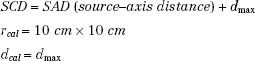
Normal incidence and open-beam geometry (i.e., absence of trays or any beam-modifying filters) are specified.

For treatment machines calibrated isocentrically, the point of MU specification is located at distance SAD rather than at distance SAD + d_max as stated previously. For isocentric calibration, SCD = SAD.

The linac is calibrated by adjusting the sensitivity of its internal monitor transmission ion chamber so that 1 MU equals 1 cGy for the reference calibration geometry condition. Several reports providing more details on monitor unit calculations and their verification are listed in the references.^22–24

MU Calculation for Fixed Fields

When the patient is to be treated isocentrically, the point of dose prescription is located at the isocenter regardless of the target depth. Using the notation of Khan et al.,⁶ the MU needed to deliver a prescribed tumor dose to isocenter (TD_iso) for a depth d of overlying tissue on the central ray is given by:

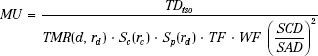
where TF and WF denote the tray and wedge factors, respectively. They are defined as the ratio of the central ray dose with the tray or wedge filter in place relative to the dose in the open-beam geometry. The collimated field size is denoted by r_c and is usually described as the square field size equivalent to the rectangular collimator opening projected to isocenter. The effective field size is denoted by r_d and is always specified to the isocenter distance (SAD). The inverse-square law factor accounts for the difference in distances from the source-to-point of dose prescription relative to the point of MU specification. When isocentric calibration is used, this factor is unity. Note that collimator-defined field size is used for lookup of the collimator scatter factor, S_c, whereas effective field size projected to isocenter is used for lookup of TMR and the phantom scatter factor, S_p. By separately accounting for the effect of collimator opening on the primary dose component and the influence of cross-sectional area of tissue irradiated, most of the difficulties in accurately delivering a dose in the presence of extensive blocking are overcome.

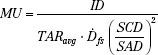
When a fixed distance between the target and entry skin surface (SSD) is used to treat the patient, a dose-calculation formalism based on PDD is used rather than one based on isocentric dose ratios. When a dose TD is to be delivered to depth d, MUs are given by:

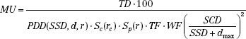
The field size (or its equivalent square) on the skin surface at central axis is denoted by r and is used for lookup of both PDD and S_p. The collimated field size r_c at the isocenter must be used for lookup of S_c. When an extended treatment distance is used, the collimated field size at isocenter differs significantly from that at the skin surface of the patient. Note that PDD is a function of SSD, depth, and effective field size. Collimator scatter factors measured at SAD are valid over a wide range of extended treatment distances.⁶

When this dose calculation formalism for highly extended treatment distances such as encountered in administering total-body irradiation is used, care must be taken to verify the validity of inverse-square law at these distances. It is recommended that such setups always be verified by ion chamber measurement at the extended distance. Because of the large scatter contribution to effective primary dose originating from the flattening filter and other components in the treatment head, the virtual source of radiation may be as much as 2 cm proximal to the target of the accelerator.

The TAR system of dose calculation is a widely used alternative to the Khan formalism. It is simply an extension of the familiar TAR and backscatter factor concepts, as used in ⁶⁰Co and orthovoltage dosimetry, to the megavoltage photon energy range. The needed dosimetry parameters are determined from ion chamber measurements (both in-phantom and in-air) like those performed for ⁶⁰Co, but now using a much larger buildup cap (radius thickness = d_max). Thus, the megavoltage peakscatter factor, PSF(r), for an effective field size r is simply the ratio of the two ion chamber readings as shown here.

And the megavoltage beam dose rate (Gy/MU) in free space, , is given by:

where the numerator is the measured d_max dose at distance SSD = SAD + d_max and collimator setting r_c. Implementation of this system requires a table of 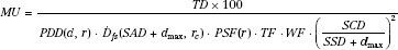values for each collimator opening and a table of PSF versus effective field size. Then, dose at d_max per MU for any distance, effective field size, and collimator opening can be calculated easily.

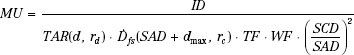
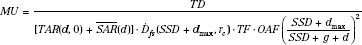
When the patient is to be treated isocentrically, the MU needed to deliver a prescribed isocenter dose (ID) to a depth d on the central axis is given by:

If the treatment is fixed SSD, the MU needed to deliver a prescribed dose (TD) to a depth d on the central ray is given by:

All MU calculation formalisms require some means of estimating the square field size, r, that is equivalent, in terms of scattering characteristics, to an arbitrary rectangular field of width a and length b. Perhaps the most widely used rectangular equivalency principle is the “A/P” rule. It states that a square and a rectangle are equivalent if they have the same area/perimeter ratio; that is:

Another widely used approach to reducing rectangular estimates of effective field size to square field sizes is the equivalent square table published in the British Journal of Radiology.²⁵ Estimating the effective field size equivalent to an irregular field is best handled via irregular field calculations as discussed later in this chapter.^26,27

MU Calculations for Asymmetric X-Ray Collimators

Asymmetric x-ray collimators (also referred to as independent jaws) allow independent movement of an individual jaw and may be available for one jaw pair or both pairs. Because MU calculations and treatment planning methods generally rely on symmetric jaw data, the dosimetric effects for asymmetric jaws must be fully documented before being implemented in the clinic. Several investigators have examined the effects of asymmetric jaws on PDD, collimator scatter, and isodose distributions.^28,29 Monitor unit calculations for asymmetric jaws are only slightly more complex than for symmetric jaws.²² Typically, one simply applies an off-axis ratio (OAR) or off-center ratio (OCR) correction factor that depends only on the distance from the machine’s central axis to the center of the independently collimated open field.^30,31 PDD is only minimally affected, but isodose curve shape can be altered and must be investigated for the particular treatment unit. Calculations for asymmetric wedge fields follow similar procedures by simply incorporating a wedge OAR or OCR.^29,32

MU Calculations for Multileaf Collimator

Multileaf collimators (MLCs) have nearly completely replaced conventional alloy field shaping for photon beams in most clinics around the world. Several investigators have examined the effects of the Varian MLC design (tertiary system) on PDD, collimator scatter, and isodose distributions.³³ The effects due to field area shaped by this type of MLC on PDD and beam output parameters are similar to those resulting from Cerrobend field shaping. Thus, the dose/MU calculation methods discussed previously apply by simply using the equivalent area defined by the MLC. The collimator scatter factor and the dose in free space are determined using the x-ray collimator jaw settings, with an off-axis factor applied for any asymmetric jaw settings.

It should be noted, however, that for MLC systems that replace one of the collimating jaws, the MLC field shape can be a determining factor in selecting the appropriate output factor.³⁴ For example, in the case of the Elekta linacs (Elekta AB, Crawley, United Kingdom), in which the lower jaws are replaced by the MLC system, the calculation takes into consideration the collective blocked area that is created by both the MLC leaves and the lower backup diaphragms.³⁵ For an MLC system that replaces the upper jaw (e.g., Siemens linac, Siemens Medical Solutions USA, Inc., Malvern, PA), Das et al.³⁶ describe a method that relies on the blocked area for determining all the calculation parameters (mainly output, percent depth dose, and scatter factor).

Hence, because of MLC design differences and the fact that vendors are continuing to modify/improve MLC designs, the authors caution that when a new linac is installed, the impact of the MLC on the institution’s MU calculation procedure should be fully documented before clinical use. The reader is also encouraged to review the AAPM Task Group 50 Report, which provides more detail on various MLC types and discusses quality assurance (QA) and MU calculations.³⁷

FIGURE 7.2. Outline of mantle field illustrating method of determining scatter-to-air ratio, used for irregular-field dose calculations. (From Cundiff JH, Cunningham JR, Golden R, et al. A method for the calculation of dose in the radiation treatment of Hodgkin’s disease. Am J Roentgenol 1973;117:30–34.)

MU Calculations for Irregular Fields

For large, irregularly shaped fields and at points off the central axis, it is necessary to take account of the off-axis change in intensity (relative to the central axis) of the beam, the variation of the SSD within the field of treatment, the influence of the primary collimator on the output factor, and the scatter contribution to the dose. Changes in the beam quality as a function of position in the radiation field also should be considered.^38,39

The general method used for irregular-field calculations consists of summation at each point of interest of the primary and scatter irradiation, with allowance for the off-axis change in intensity (off-axis factor) and SSD.^26,27 The MUs required to deliver a specified tumor dose at an arbitrary point in an irregular field (Fig. 7.2) can be calculated as follows:

where the parameters used are:

Computer implementations vary, but typically include using the expanded field size at a depth for the SAR calculation, determining the off-axis factor using the distance from the central axis to the slant projection of the point of calculation to the SSD plane along a ray from the source, and determining the zero-area TAR using the slant depth along a ray going from the source to the point of calculation. It is generally accepted that the off-axis factor should be multiplied by the sum of the zero-area TAR and the SAR as originally proposed.

Beam quality is a function of position in the field for beams generated by linear accelerators.^38,39 The TAR₀ may be expressed as a function of position in the beam so that changes in beam quality can be incorporated into calculations, and it can be related to the half-value layer (HVL) of water by the following equation:

where d is the depth of the point of reference, d_max is the depth of maximum dose, r is the radial distance from the central axis of the beam to the point of calculation, e is the base of the natural logarithm, and HVL(r) is the beam quality expressed as the HVL measured in water.

MU Calculations for Rotation Therapy

The classic method for MU calculations for rotation therapy is given by the following equation:

and the MU per degree setting is given by:

where the symbols have the previous meaning and TAR_avg is an average TAR (averaged over radii [depth in the patient] at selected angular intervals, such as 10 or 20 degrees).

Most recently, manufacturers of linacs and their associated planning systems have introduced features that provide rotational intensity modulated radiation therapy (IMRT) capability^40,41 (e.g., Elekta VMAT⁴² and Varian RapidArc⁴³). The linac-based rotational IMRT concept was first proposed by Yu^44,45 and called intensity modulated arc therapy (IMAT), but planning software was not commercially available at that time. Rotational IMRT approaches on conventional linacs may provide even more conformal dose distributions delivered in a shorter treatment time, compared with SMLC-IMRT (step and shoot) or DMLC-IMRT (dynamic) approaches that use only a limited number of gantry directions. In addition, plan optimization is simpler because it eliminates the planner’s iterative choices of beam number and direction. The conventional MLC approach for rotational IMRT is likely to improve IMRT plan quality and delivery efficiency,⁴³ although this remains somewhat controversial at present^46,47 and more users will need to report their rotational IMRT experiences over the next few years. Monitor unit calculations for this more complex form of rotational therapy are generated via advanced treatment planning systems having this capability. All are techniques in which the MLC shape changes during a rotation therapy, and depending on the specific linac, other parameters, such as dose rate, may also change. This advanced type of treatment delivery is currently checked via phantom measurements rather than manual calculations prior to the patient’s treatment.

It is apparent that the simple MU manual calculations methods described here are no longer adequate for the complex technologies in use today. Modern computer plans utilize dose weight points of interest, which classical MU calculation methods may not address; in addition, geometries that include the presence of heterogeneities, added tertiary devices such as MLCs and asymmetric jaws, and beam intensity modulation can all be problematic for manual check calculations. For example, when the dose weight point is within a small volume of mass surrounded by low-density tissue (e.g., a coin lesion in lung) or one that is at the border of a chest wall and lung (as in a postmastectomy patient), MU calculations cannot easily be confirmed by simple hand-calculated MU methods, and one must rely on the planning system for calculations such as these, emphasizing the importance of fully testing such system prior to clinical use. Dedicated commercial software for MU verification is now available, for example, RadCalc (LifeLine Software Inc, Austin, TX) based on the work of Kung et al.⁴⁸ and IMSure (Standard Imaging, Middleton, WI) based on the work of Yang et al.⁴⁹ Obviously such systems must also be validated by the physics user prior to clinical use.

FIGURE 7.3. Typical photon and electron beam central-axis percentage depth dose (DD) curves for a 10 × 10 cm beam for megavoltage beams ranging from ⁶⁰Co to 18-MV x-rays and 6- to 20-MeV electron beams.

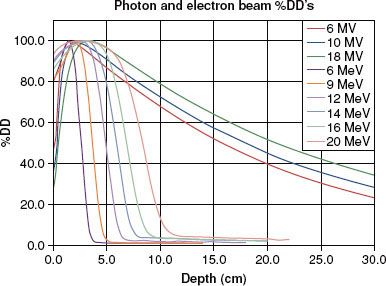
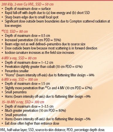
TABLE 7.1 BEAM CHARACTERISTICS FOR PHOTON BEAM ENERGIES OF INTEREST IN RADIATION THERAPY

CLINICAL PHOTON BEAM DOSIMETRY

Percent Depth Dose and Single-Field Isodose Charts

The central-axis PDD expresses the penetrability of a radiation beam. Table 7.1 summarizes beam characteristics for x-ray and γ-ray beams typically used in radiation therapy and lists the depth at which the dose is maximum (100%) and the 10-cm depth PDD value. Representative PDD curves are shown in Figure 7.3 for conventional SSDs. As a rule of thumb, an 18-MV, 6-MV, and ⁶⁰Co photon beam loses approximately 2%, 3.5%, and 4.5% per centimeter, respectively, beyond the depth of maximum dose, d_max (values are for a 10 × 10 cm field, 100-cm SSD). There is no agreement as to what is the single optimal x-ray beam energy; instead, institutional bias or radiation oncologist training typically influences its selection, and it is usually treatment site specific. As pointed out in Chapter 5, most modern linacs are multimodality, and provide a range of photon and electron beam energies ranging from 4 to 25 MV, with 6- and 15 or 18-MV x-ray beams the most common.

Isodose charts provide much more information about the radiation beam characteristics than do central-axis PDD data alone. However, even isodose charts are limited in that they represent the dose distribution in only one plane (typically the one containing the beam’s central axis) and are usually available only for square or rectangular fields. Isodose charts are usually measured in a water phantom with the radiation beam directed perpendicular to the phantom’s flat surface. Isodose curves show the relative uniformity of the beams across the field at various depths, and also provide a graphical depiction of the width of the beam’s penumbra region. ⁶⁰Co teletherapy units exhibit a relatively large penumbra, and their isodose distributions are more rounded than those from linac x-ray beams. This is due to the relatively large source size (typically 1 to 2 cm in diameter vs. only a few millimeters for linacs). Linac beam penumbra width does increase slightly as a function of energy and if unfocused MLC leaves are used, but is still much less than that for ⁶⁰Co units. In addition to the smaller penumbra, linac x-ray isodose distributions have relatively flat isodose curves at depth. However, at shallow depths, particularly at d_max, linac x-ray beams typically exhibit an increase in beam intensity away from the central axis; this beam characteristic is referred to as the dose profile horns and depends on flattening filter design. In general, each treatment unit has unique radiation beam characteristics, and thus, isodose distributions must be measured, or at least verified, for each specific treatment unit.

Another important point to understand is how the radiation field size is defined. The radiation field size dimensions refer to the distance perpendicular to the beam’s direction of incidence that corresponds to the 50% isodose at the beam’s edge. It is defined at the skin surface for SSD treatments, and at the SAD for isocentric treatments.

FIGURE 7.4. Relative surface dose versus field size with blocking tray in place for 6- and 18-MV photons. (From Klein EE, Purdy JA. Entrance and exit dose regions for Clinac-2100 C. Int J Radiat Oncol Biol Phys 1993;27:429–435.)

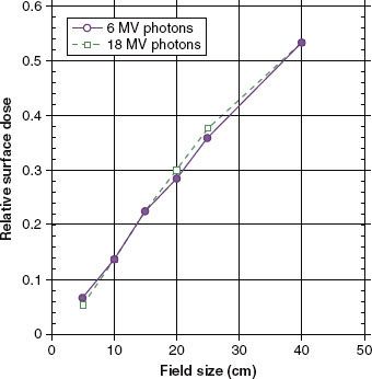
FIGURE 7.5. The variation of surface dose and depth of maximum dose as a function of the angle of incidence of the x-ray beam with the surface (4 MV, 10 × 10 cm).

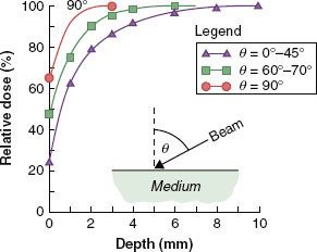
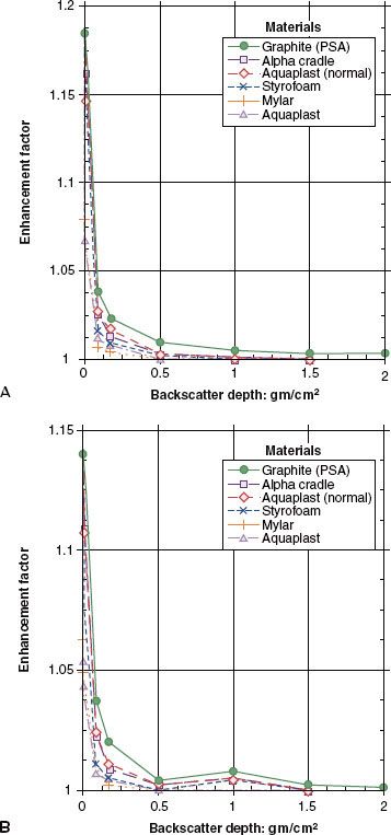
FIGURE 7.6. Enhancement of exit dose for (A) 6-MV and (B) 18-MV photons for a 15 × 15 cm field at 100-cm source-to-axis distance versus backscatter depth for various backscattering materials. (From Klein EE, Purdy JA. Entrance and exit dose regions for Clinac-2100 C. Int J Radiat Oncol Biol Phys 1993;27:429–435.)

Depth-Dose Buildup Region

When a photon beam strikes the tissue surface, electrons are set in motion, causing the dose to increase with depth until the maximum dose is achieved at depth d_max. As the energy of the photon beam increases, the thickness of the buildup region is increased. The subcutaneous tissue-sparing effects of higher-energy x-rays, combined with their great penetrability, make them well suited for treating deep lesions. In general, the dose to the surface and in the buildup region for megavoltage photon beams generally increases with increasing field size and with the insertion of blocking trays made of plastic or other type material in the beam (Fig. 7.4). The blocking trays should be at least 20 cm above the skin surface because skin doses are significantly increased for lesser distances. Copper, lead, or lead glass filters beneath the blocking tray can be used to remove the undesired lower-energy electrons that contribute to skin dose, but this is nowadays rarely done routinely in the clinic.^50,51

As the angle of the incident radiation beam becomes more oblique, the surface dose increases, and d_max moves toward the surface (Fig. 7.5). This is primarily due to more secondary electrons’ contribution from the media below the surface along the oblique path of the beam.⁵²

Depth Dose/Exit Dose Region

The skin and superficial tissue on the side of the patient from which the beam exits receive a reduced dose if there is insufficient backscatter material present. The amount of dose reduction is a function of x-ray beam energy, field size, and the thickness of tissue that the beam has penetrated reaching the exit surface. For a 6-MV beam, a 15% reduction in dose with little dependency on field size has been reported,⁵⁰ and for 18-MV beams, an 11% reduction in exit dose was measured.⁵³ In general, the addition of a thickness of tissue-equivalent material on the exit side equivalent in thickness to approximately two-thirds of the d_max depth is sufficient to provide full dose to the build-down region on the exit side. Figure 7.6 shows the effects of various backscattering media when placed directly behind the exit surface.

Tissue Heterogeneities and Tissue Interface Dosimetry

The presence of tissue heterogeneities, such as air cavities, lungs, bony structures, and prostheses, can greatly impact the calculated dose distribution. The change in dose is due to the perturbation of the transport of primary and scattered photons and that of the secondary electrons set in motion from photon interactions. Depending on the energy of the photon beam and the shape, size, and constituents of the inhomogeneities, the resultant change in dose can be large.

Perturbation of photon transport is more noticeable for lower-energy beams. There is usually an increase in transmission, and therefore dose, when the beam traverses a low-density inhomogeneity. The reverse applies when the inhomogeneity has a density higher than that of water. However, the change in dose is complicated by the concomitant decrease or increase in the scatter dose. For a modest lung thickness of 10 cm, there will be about a 15% increase in the dose to the lung for a ⁶⁰Co or 6-MV x-ray beam, but only about 5% for an 18-MV x-ray beam.⁵⁴

When there is a net imbalance of electrons leaving and entering the region near an inhomogeneity (interfaces of different media), the condition of electron equilibrium is disrupted. The dose distribution in the patient in such transition zones depends on radiation field size (scatter influence), distance between interfaces (e.g., air cavities), differences between physical densities and atomic number of the interfacing media, and the size and shape of the different media. Because electrons have finite travel, the resultant change in dose is usually local to the vicinity of the inhomogeneity but may be quite large. The effects are more noticeable for the higher photon energy beams due to the increased energy and range of the scattered electrons. Near the edge of the lungs and air cavities, the reduction in dose can be larger than 15%.⁵⁵

For inhomogeneities with density larger than water, there will be an increase in dose locally due to the generation of more electrons. However, most dense inhomogeneities have atomic numbers higher than that of water so that the resultant dose perturbation is further compounded by the perturbation of the multiple coulomb scattering of the electrons. Near the interface between a bony structure and waterlike tissue, large hot and cold dose spots can be present. Several benchmark measurements have been reported for various geometries simulating clinical situations and are discussed briefly in the following sections.

Air Cavities

Air cavities that appear in various locations of the body, most particularly in the head and neck region, pose a problem due to loss of equilibrium at the air–tissue boundaries internal to the patient. Epp et al.⁵⁶ reported that for cobalt beams, a reduction in dose of approximately 12% was found for a typical larynx air cavity, which recovered within 5 mm in the new buildup region. The loss was due to a lack of forward scattered electrons. Epp et al.⁵⁷ reported that for a 10-MV x-ray beam, a 14.5% loss was measured at the distal interface of the air cavity with a buildup curve that plateaued within 20 mm of the interface. Klein et al.⁵⁸ measured distributions about air cavities for 4-MV and 15-MV x-ray beams in both the distal and proximal regions. The combined dose distribution in a parallel-opposed fashion showed a 10% loss at the interfaces for both beam energies.

Lung Tissue

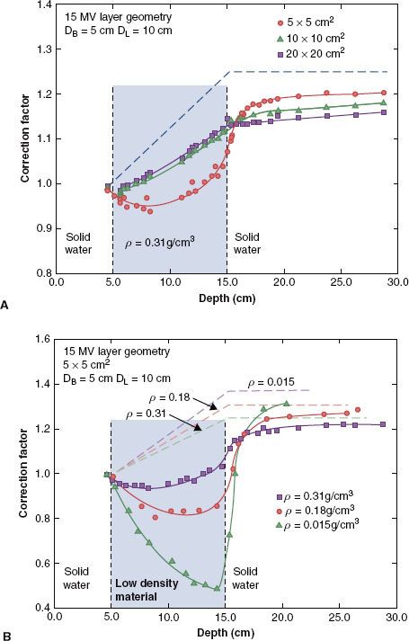
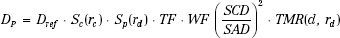
Although the problem of reestablishing equilibrium for lung interfaces is not as severe as with air cavities, a transition zone region at the lung–tissue interface still exists over the range of typical clinical photon beam energies. Rice et al. measured responses within various simulated lung media for 4-MV and 15-MV x-rays using a parallel-plate ion chamber and a phantom constructed of solid water and simulated lung material (average lung material density, ρ = 0.31 g/cm³; some additional measurements made with materials having densities of 0.015 g/cm³ and 0.18 g/cm³).⁵⁹ Figure 7.7 shows the results in terms of measured CFs for the 15-MV beam. A considerable buildup curve was observed (10% change in CF) for small fields (5 × 5 cm²) for the 15-MV beam, which began in the distal region of the lung and plateaued about 5 cm beyond the simulated lung interface.

Bone–Soft Tissue Interfaces

Das et al.⁶⁰ measured dose perturbation factors (DPFs) proximal and distal for simulated bone–tissue interface regions using a parallel-plate chamber for both 6- and 24-MV x-ray beams. They reported DPFs of 1.1 for the 6-MV beam and 1.07 for the 24-MV beam at the proximal interface. At the distal interface, a DPF of 1.07 was measured for the 24-MV beam, whereas the 6-MV beam exhibited a DPF of 0.95, resulting in a new buildup region in soft tissue. Note, both buildup and build-down regions dissipate within a few millimeters from the interfaces and the perturbations are independent of thickness and lateral extent of the bone or radiation field size.

Metal Prostheses

Das and associates measured DPFs following a 10.5-mm-thick stainless steel layer simulating a hip prosthesis geometry.⁶⁰ They reported a DPF of 1.19 for 24-MV photons, but only 1.03 for 6-MV photons; on the proximal side, they reported a DPF of 1.30 due to the backscattered electrons that was independent of energy, field size, or lateral extent of the steel. These interface effects dissipated within a few millimeters in polystyrene. Other reports dealing with dosimetry perturbations due to metal objects are included in the references.^61,62

Niroomand-Rad et al. reported on dose perturbation effects at the tissue–titanium alloy implant interfaces in patients with head and neck cancer treated with 6-MV and 10-MV photon beams.⁶³ They found at the upper surface (toward the source) of the tissue–dental implant interface DPFs of 1.22 and 1.20 for the 6-MV and 10-MV photon beams, respectively. At the lower interface, dose reduction was approximately −13.5% and −9.5% for the 6-MV and 10-MV beams, respectively.

The most complete information currently available on hip prosthesis dosimetry is found in AAPM Report 81 (TG 63).⁶⁴ The report provides the current state of scientific understanding and clinical dosimetry in use for patients with high-Z hip prostheses undergoing radiation therapy. Beam arrangements that avoid the prosthesis should always be a first consideration. If this cannot be done, valuable information is available in Report 81, including values for different prostheses’ electron density, approximate attenuation of the beam passing through the prosthesis, and possible dose increase to the hip bone. It should also be noted that some of the data provided and recommendations are also applicable to patients having other implanted high-Z prosthetic devices such as pins and humeral head replacements.

Silicone–Soft Tissue Interfaces

Klein and Kuske reported on interface perturbations with silicon breast prostheses.⁶⁵ Such prostheses have a density similar to breast tissue but have a different atomic number. They observed a 6% enhancement at the proximal interface and a 9% loss at the distal interface.

Wedge Filter Dosimetry

When a wedge filter is inserted into the beam, the dose distribution is angled at some specified depth to some desired angle relative to the incident beam direction over the entire transverse dimension of the radiation beam (Fig. 7.8). For cobalt units, the depth of the 50% isodose usually is selected for specification of the wedge angle, whereas for high-energy linacs, higher-percentile isodose curves, such as the 80% curve, or the isodose curves at a specific depth (10 cm) are used to define the wedge angle.

Linacs are typically equipped with multiple wedges that may be used with an allowed range of field sizes. Although linac wedges can be designed for any desired wedge angle, 15-, 30-, 45-, and 60-degree wedges are the most common.

FIGURE 7.7. A: Dose correction factors as a function of depth for a transition zone geometry that simulates a lung–tissue interface for three different field sizes and a lung thickness of 10 cm for 15-MV x-rays. The modification to the primary dose only on the central axis (shown by the dashed curve) is independent of field size. B: Dose correction factors as a function of depth for a transition zone geometry that simulates a lung–tissue interface for three different densities, a 5 × 5 cm field, and a lung thickness of 10 cm for 15-MV x-rays. The modification to the primary dose only on the central axis is shown by the dashed curve. (From Rice RK, Mijnheer BJ, Chin LM. Benchmark measurements for lung dose corrections for x-ray beams. Int J Radiat Oncol Biol Phys 1988;15:399–409.)