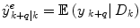
at time k is formed by a linear weighted average of the individual predictors  .
.

(1)
A special case, considering distinct switches between different linear system dynamics, has been studied mainly in the control community. The data stream and the underlying dynamic system are modelled by pure switching between different filters derived from these models, i.e., the weights w k can only take value 1 or 0. A lot of attention has been given to reconstructing the switching sequence, see, e.g., [47, 73]. From a prediction viewpoint, the current dynamic mode is of primary interest, and it may suffice to reconstruct the dynamic mode for a limited section of the most recent time points in a receding horizon fashion [4].
Combinations of specifically adaptive filters has also stirred some interest in the signal processing community. Typically, filters with different update pace are merged, to benefit from each filter’s specific change responsiveness, respectively steady state behaviour [5].
Finally, in fuzzy modeling, soft switching between multiple models is offered using fuzzy membership rules in the Takagi–Sugeno systems [100].
Merging of predictions in the glucose prediction context has previously been investigated in terms of hypo- or hyperglycemic warning systems. In [25], the glucose prediction from a so-called output corrected ARX predictor (see the reference for method details) was linearly combined with the prediction from an adaptive recurrent neural network model. The balancing factor for the linear combination was determined offline by optimizing a trade-off between hypo- and hyperglycemic sensitivity, effective prediction horizon and the false alarm rate. This factor was determined individually for each patient and the balance may be different for hypo- and hyperglycemia. A different mechanism was used in [27]. Here, five different predictors were running simultaneously, and the hypoglycemic alarm was based upon a voting scheme between the individual predictors. If a number of the five predictors exceeded the predefined hypoglycemic threshold value an alarm was raised. Both studies indicated an improvement in alarm sensitivity compared to the individual predictors.
2 Problem Formulation
As seen from the review above, many different approaches to glucose modeling and predicting have been established. These methods may each be more suitable to specific conditions for the glucose dynamics, and improvements in robustness and prediction performance may be achieved by combining their outcomes, as indicated from the studies from the hypo-/hyperglycemic alarm systems. Such a situation is depicted in Fig. 1, where two prediction models try to capture the true glucose level. In different situations, each predictor is clearly outperforming the other and is capable of providing good estimates of the true glucose level. However, as the conditions change the performance deteriorates, and instead the other predictor is more suitable to rely upon. Given this informal background a more formal problem formulation is now outlined.
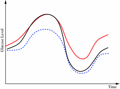
Fig. 1
Example of when merging between different predictors may be beneficial. Initially the model corresponding to the red dash-dotted prediction resembles the true reference (black solid curve) best, but as the conditions change the prediction given by the other prediction model (blue dashed curve) gradually takes the lead
A non-stationary data stream  arrives with a fixed sample rate, set to 1 for notational convenience, at time
  The data stream contains a variable of primary interest called
  and additional variables u k . The data stream can be divided into different periods
  of similar dynamics
 ![$$S_{i} \in S = \left[ {1, \ldots ,n} \right],$$](/wp-content/uploads/2017/04/A310669_1_En_2_Chapter_IEq7.gif) and where s k ∈ S indicates the current dynamic mode at time t k . The system changes between these different modes according to some unknown dynamics.
and where s k ∈ S indicates the current dynamic mode at time t k . The system changes between these different modes according to some unknown dynamics.
arrives with a fixed sample rate, set to 1 for notational convenience, at time The data stream contains a variable of primary interest called and additional variables u k . The data stream can be divided into different periods of similar dynamics and where s k ∈ S indicates the current dynamic mode at time t k . The system changes between these different modes according to some unknown dynamics.Given m number of expert q-steps-ahead predictions,  of the variable of interest at time t k , each utilizing different methods, and/or different training sets; how is an optimal q-steps-ahead prediction
  of the primary variable, using a predefined norm and under time-varying conditions, determined?
of the variable of interest at time t k , each utilizing different methods, and/or different training sets; how is an optimal q-steps-ahead prediction of the primary variable, using a predefined norm and under time-varying conditions, determined?3 Sliding Window Bayesian Model Averaging
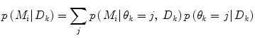
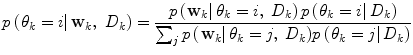
Apart from conceptual differences between the different approaches to ensemble prediction, the most important difference is how the weights are determined. Numerous different methods exist, ranging from heuristic algorithms [5, 100] to theory based approaches, e.g., [49]. Specifically, in a Bayesian Model Averaging framework [49], which will be adopted in this chapter, the weights are interpreted as partial beliefs in each predictor M i , and the merging is formulated as:
where  is the conditional probability of y at time t k+q given the data,
  received up until time k, and if only point-estimates are available, one can, e.g., use:
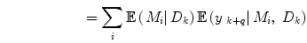

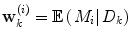
where  is the combined prediction of
  using information available at time k, and
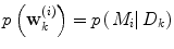
  indicates position i in the weight vector. The conditional probability of predictor M i can be further expanded by introducing the latent variable
 ![$$\theta_{k} \in \varTheta = \left[ {1, \ldots ,p} \right].$$](/wp-content/uploads/2017/04/A310669_1_En_2_Chapter_IEq15.gif)
or in matrix notation
![$${\mathbf{p}}\left( {{\mathbf{w}}_{k} } \right) = \left[ {{\mathbf{p}}\left( {\left. {{\mathbf{w}}_{k} } \right|\theta_{k} = 1} \right), \ldots ,{\mathbf{p}}\left( {\left. {{\mathbf{w}}_{k} } \right|\theta_{k} = p} \right)} \right]\;\left[ {p\left( {\left. {\theta_{k} = 1} \right|D_{k} } \right), \ldots ,p\left( {\left. {\theta_{k} = p} \right|D_{k} } \right)} \right]^{T}$$](/wp-content/uploads/2017/04/A310669_1_En_2_Chapter_Equ9.gif)
(2)
is the conditional probability of y at time t k+q given the data, received up until time k, and if only point-estimates are available, one can, e.g., use:(3)
(4)
(5)
(6)
(7)
is the combined prediction of using information available at time k, and indicates position i in the weight vector. The conditional probability of predictor M i can be further expanded by introducing the latent variable (8)
(9)
Here,  represents a predictor mode in a similar sense to the dynamic mode S, and likewise
  represents the prediction mode at time
 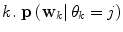 is a column vector of the joint prior distribution of the conditional weights of each predictor model given the predictor mode
  . Generally, there is a one-to-one relationship between the predictor modes and the corresponding dynamic modes, i.e., p = n.
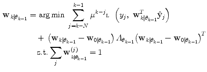
represents a predictor mode in a similar sense to the dynamic mode S, and likewise represents the prediction mode at time is a column vector of the joint prior distribution of the conditional weights of each predictor model given the predictor mode . Generally, there is a one-to-one relationship between the predictor modes and the corresponding dynamic modes, i.e., p = n. Data for estimating the distribution for 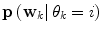 is given based upon using a constrained optimization on the training data. In cases of labelled training data sets, the following applies:
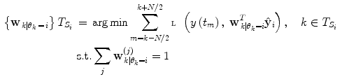
where  represents the time points corresponding to dynamic mode S i , the tunable parameter N determines the size of the evaluation window and
  is a cost function. From these data sets, the prior distributions can be estimated by the Parzen window method [11], giving mean
  and covariance matrix
  . An alternative to the Parzen approximation is of course to estimate a more parsimoniously parametrized probability density function (pdf) (e.g., Gaussian) for the extracted data points. For unlabelled training data, with time points T, the corresponding datasets
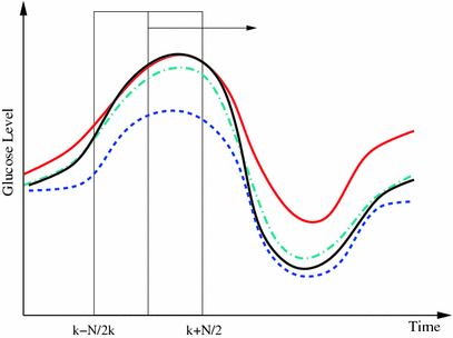
 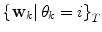 are found by cluster analysis, e.g., using the k-means algorithm or a Gaussian Mixture Model (GMM) [11]. A conceptual visualisation is given in Fig. 2. Now, in each time step k, the
  is determined from the sliding window optimization below, using the current active mode
  . For reasons soon explained, only
  is thus calculated:
Here, μ j is a forgetting factor, and  is a regularization matrix. To infer the posterior
  in (9), it would normally be natural to set this probability function equal to the corresponding posterior pdf for the dynamic mode
  . However, problems arise if
  is not directly possible to estimate from the dataset D k . This is circumvented by using the information provided by the
  estimated from the data retrieved from Eq. (10) above. The
  prior density functions can be seen as defining the region of validity for each predictor mode. If the
  estimate leaves the current active mode region
  (in a sense that
  is very low), it can thus be seen as an indication of that a mode switch has taken place. A logical test is used to determine if a mode switch has occurred. The predictor mode is switched to mode
  , if:
, if:
A λ somewhat larger than 0.5 gives a hysteresis effect to avoid chattering between modes. Unless otherwise estimated from data, the conditional probability of each prediction mode 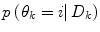 is set equal for all possible modes, and thus cancels in (13). The logical test is evaluated using the priors received from the pdf estimate and the
  received from (11). If a mode switch is considered to have occurred (11) is rerun using the new predictor mode.
is given based upon using a constrained optimization on the training data. In cases of labelled training data sets, the following applies:(10)
represents the time points corresponding to dynamic mode S i , the tunable parameter N determines the size of the evaluation window and is a cost function. From these data sets, the prior distributions can be estimated by the Parzen window method [11], giving mean and covariance matrix . An alternative to the Parzen approximation is of course to estimate a more parsimoniously parametrized probability density function (pdf) (e.g., Gaussian) for the extracted data points. For unlabelled training data, with time points T, the corresponding datasets are found by cluster analysis, e.g., using the k-means algorithm or a Gaussian Mixture Model (GMM) [11]. A conceptual visualisation is given in Fig. 2. Now, in each time step k, the is determined from the sliding window optimization below, using the current active mode . For reasons soon explained, only is thus calculated:Fig. 2
Principle of finding the predictor modes for unlabelled data over the training data set time period T. For every time point t k ∈ T, the optimal w k is determined by Eq. (10), where the optimal prediction  (light green dash-dotted curve) formed from the individual predictions
  (the blue dashed and the red solid curves) is evaluating against the reference (black solid curve) using the cost function
  over a sliding data window between t = k − N/2 and t = k + N/2. The aggregated set {w k } T is thereafter subjected to clustering to find the different mode centers
 ![$${\mathbf{w}}_{\left. 0 \right|\theta = i} ,\;i = \left[ {1, \ldots ,p} \right]$$](/wp-content/uploads/2017/04/A310669_1_En_2_Chapter_IEq73.gif)
(light green dash-dotted curve) formed from the individual predictions (the blue dashed and the red solid curves) is evaluating against the reference (black solid curve) using the cost function over a sliding data window between t = k − N/2 and t = k + N/2. The aggregated set {w k } T is thereafter subjected to clustering to find the different mode centers (11)
is a regularization matrix. To infer the posterior in (9), it would normally be natural to set this probability function equal to the corresponding posterior pdf for the dynamic mode . However, problems arise if is not directly possible to estimate from the dataset D k . This is circumvented by using the information provided by the estimated from the data retrieved from Eq. (10) above. The prior density functions can be seen as defining the region of validity for each predictor mode. If the estimate leaves the current active mode region (in a sense that is very low), it can thus be seen as an indication of that a mode switch has taken place. A logical test is used to determine if a mode switch has occurred. The predictor mode is switched to mode , if:(13)
is set equal for all possible modes, and thus cancels in (13). The logical test is evaluated using the priors received from the pdf estimate and the received from (11). If a mode switch is considered to have occurred (11) is rerun using the new predictor mode.Now, since only one prediction mode θ k is active; (9) reduces to 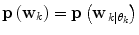 . The predictor mode switching concept is visualised in Fig. 3.
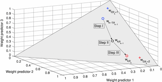
. The predictor mode switching concept is visualised in Fig. 3.Fig. 3
Predictor mode switching for an example with three individual predictor models. Step I At time instance t k the new  is determined from Eq. (11) In this case, the data forces the optimal weight away from the active prediction mode center. Step II The likelihood values
 ![$$p\left( {\left. {w_{k} } \right|\theta_{k} = i} \right),\;i = \left[ {1, \ldots ,p} \right]$$](/wp-content/uploads/2017/04/A310669_1_En_2_Chapter_IEq75.gif) are calculated and if the condition according to Eq. (12) is fulfilled, a predictor mode switch occurs. Step III Based on the new predictor mode, Eq. (11) is rerun and the weight vector now gravitates towards the new mode center
are calculated and if the condition according to Eq. (12) is fulfilled, a predictor mode switch occurs. Step III Based on the new predictor mode, Eq. (11) is rerun and the weight vector now gravitates towards the new mode center
is determined from Eq. (11) In this case, the data forces the optimal weight away from the active prediction mode center. Step II The likelihood values are calculated and if the condition according to Eq. (12) is fulfilled, a predictor mode switch occurs. Step III Based on the new predictor mode, Eq. (11) is rerun and the weight vector now gravitates towards the new mode center3.1 Parameter Choice
The length N of the evaluation period is, together with the forgetting factor μ, a crucial parameter determining how fast the ensemble prediction reacts to sudden changes in dynamics. A small forgetting factor will put much emphasis on recent data, making it more agile to sudden changes. However, the drawback is of course that the noise sensitivity increases.
 should also be chosen, such that a sound balance between flexibility and robustness is found, i.e., a too small
  may result in over-switching, whereas a too large
  will give a stiff and inflexible predictor. Furthermore,
  should force the weights to move within the perimeter defined by p(w|θ k = i). This is approximately accomplished by setting
  equal to the inverse of the covariance matrix
  , thus representing the pdf as a Gaussian distribution in the regularization.
Optimal values for N and μ can be found by evaluating different choices for some test data. However, from our experience we have seen that N = 10–20 and μ = 0.8 are suitable choices for this application.
3.2 Nominal Mode
Apart from the estimated prediction mode centres, an additional predictor mode can be added, corresponding to a heuristic fall-back mode. In the case of sensor failure, or other situations where loss of confidence in the estimated predictor modes arises, each predictor may seem equally valid. In this case, a fall-back mode to resort to may be the equal weighting. This is also a natural start for the algorithm. For these reasons, a nominal mode θ k = 0 : p(w k |θ k = 0) ∈ N(1/m, I) is added to the set of predictor modes.
Summary of algorithm
1.
Estimate m numbers of predictors according to best practice.
2.
Run the predictors and the constrained estimation (10) on labelled training data and retrieve the sequence of 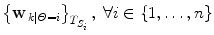 .
.
.3.
Classify different predictor modes, and determine density functions  for each mode Θ = i from the training results by supervised learning. If possible; estimate p(Θ = i|D).
for each mode Θ = i from the training results by supervised learning. If possible; estimate p(Θ = i|D).4.
Initialize mode to the nominal mode.
6.
7.
Go to 5.
The ensemble engine outlined above will hereafter be referred to as Sliding Window Bayesian Model Averaging (SW-BMA) Predictor.
4 Choice of Cost Function 
The cost function should be chosen with the specific application in mind. A natural choice for interpolation is the 2-norm, but in certain situations asymmetric cost functions are more appropriate. For the glucose prediction application, a suitable candidate for determining appropriate weights should take into account that the consequences of acting on too high glucose predictions in the lower blood glucose (G) region (<90 mg/dl) could possibly be life threatening. The margins to low blood glucose levels, that may result in coma and death, are small, and blood glucose levels may fall rapidly. Hence, much emphasis should be put on securing small positive predictive errors and sufficient time margins for alarms to be raised in due time in this region. In the normoglycemic region (here defined as 90–200 mg/dl), the predictive quality is of less importance. This is the glucose range that healthy subjects normally experience, and thus can be considered, from a clinical viewpoint in regards to possible complications, a safe region. However, due to the possibility of rapid fluctuation of the glucose into unsafe regions, some considerations of predictive quality should be maintained.
Based on the cost function in [58], the selected function incorporates these features; asymmetrically increasing cost of the prediction error depending on the absolute glucose value and the sign of the prediction error.
In Fig. 4 the cost function can be seen, plotted against relative prediction error and absolute blood glucose value.
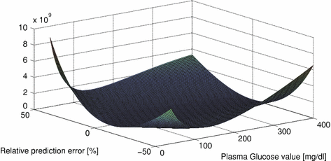
Fig. 4
Cost function of relative prediction error
4.1 Correspondence to the Clarke Grid Error Plot
A de facto accepted standardized metric of measuring the performance of CGM signals in relation to reference measurements, and often used to evaluate glucose predictors, is the Clarke Grid Plot [19]. This metric meets the minimum criteria raised earlier. However, other aspects makes it less suitable; no distinction between prediction errors within error zones is made, switches in evaluation score are instantaneous, etc.
In Fig. 5, the isometric contours of the chosen function for different prediction errors at different G values has been plotted together with the Clarke Grid Plot. The boundaries of the A/B/C/D/E areas of the Clarke Grid can be regarded as lines of isometric cost according to the Clarke metric. In the figure, the isometric value of the cost function has been chosen to correspond to the lower edge, defined by the intersection of the A and B Clarke areas at 70 mg/dl. Thus, the area enveloped by the isometric border can be regarded as the corresponding A area of this cost function.
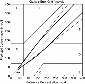
Fig. 5
Isometric cost in comparison to the Clarke Grid
Apparently, much tougher demands are imposed both in the lower and upper glucose regions in comparison to the Clarke Plot.
5 Example I: The UVa/Padova Simulation Model
5.1 Data
Data were generated using the nonlinear metabolic simulation model, jointly developed by the University of Padova, Italy and University of Virginia, U.S. (UVa) and described in [24], with parameter values obtained from the authors. The model consists of three parts that can be separated from each other. Two sub models are related to the influx of insulin following an insulin injection and the rate of appearance of glucose from the gastro-intestinal tract following meal intake, respectively.
The transport of rapid-acting insulin from the subcutaneous injection site to the blood stream was based on the compartment model in [23, 24], as follows.
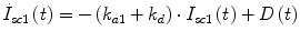
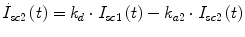

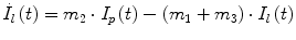
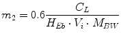
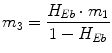
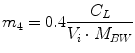
Following the notation in [23, 24], I sc1 is the amount of non-monomeric insulin in the subcutaneous space, I sc2 is the amount of monomeric insulin in the subcutaneous space, k d is the rate constant of insulin dissociation, k a1 and k a2 are the rate constants of non-monomeric and monomeric insulin absorption, respectively, D(t) is the insulin infusion rate, I p is the level of plasma insulin, I l the level of insulin in the liver, m 3 is the rate of hepatic clearance, and m 1, m 2, m 4 are rate parameters. The parameters m 2, m 3, m 4 are determined based on steady-state assumptions—relating them to the constants in Table 1 and the body weight M BW .
(14)
(15)
(16)
(17)
(18)
(19)
(20)
Table 1
Generic parameter values used for the GSM and ISM
Parameter | Value | Unit | Parameter | Value | Unit |
|---|---|---|---|---|---|
k gri | 0.0558 | [min−1] | k a1 | 0.004 | [min−1] |
k max | 0.0558 | [min−1] | k a2
Related posts: Models for In-Silico Evaluation of Closed-Loop Insulin Delivery Systems in Type 1 Diabetes
Parameters Describing Gut Absorption and Lipid Dynamics in Relation to Glucose Metabolism During a Routine Oral Glucose Test
Modeling of the Dynamic Effects of Free Fatty Acids on Insulin Sensitivity
Modeling of Diabetes Progression
Prevention Using Low Glucose Suspend Systems
and Minimal-Type Compartmental Insulin-Glucose Models: Theory and Applications Models for In-Silico Evaluation of Closed-Loop Insulin Delivery Systems in Type 1 Diabetes
Parameters Describing Gut Absorption and Lipid Dynamics in Relation to Glucose Metabolism During a Routine Oral Glucose Test
Modeling of the Dynamic Effects of Free Fatty Acids on Insulin Sensitivity
Modeling of Diabetes Progression
Prevention Using Low Glucose Suspend Systems
and Minimal-Type Compartmental Insulin-Glucose Models: Theory and Applications
Stay updated, free articles. Join our Telegram channel
Full access? Get Clinical Tree
 Get Clinical Tree app for offline access

|