. In tomography, the voxel value in a transverse slice is reconstructed from different LORs passing through all the voxels of this slice. As a result, the noise in a voxel is correlated to the noise present elsewhere in the slice [79, 80], and its order of magnitude is about that of the noise present in a projection. This explains why, although tomography provides much more information by removing the activity superimposition, the image (Fig. 8.1d) appears less natural than planar views (Fig. 8.1a–c). This also explains why much longer acquisition time is required in tomography than in planar acquisition.
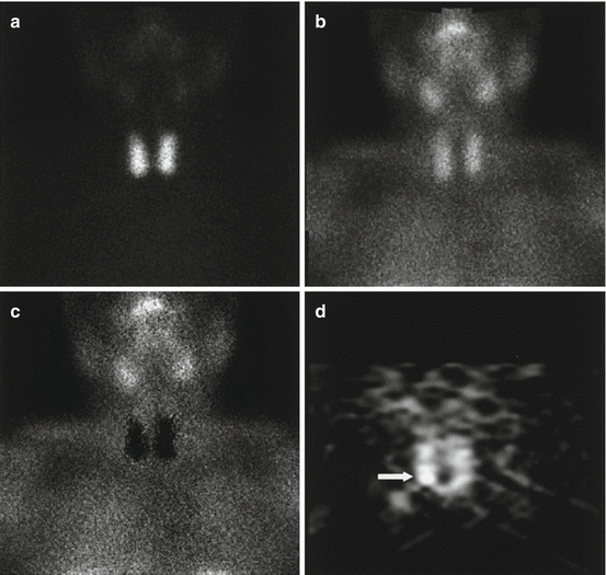
Fig. 8.1
A 55-year-old female patient affected by pHPT with small parathyroid adenoma (size, 6.1 mm; weight, 261 mg) sited behind inferior pole of right thyroid lobe, negative on planar 99mTc-pertechnetate (a), 99mTc-tetrofosmin (b) and subtraction (c) scintigraphy and clearly revealed (arrow) on coronal P-SPECT (d) (Reprinted from Spanu et al. [95] with permission of the Society of Nuclear Medicine)
8.2.2 Tomography is an Ill-Posed Problem
Let’s study the theoretical case of an ideal tomography (i.e. no disturbing physical effects) with continuous reconstruction variable (i.e. very small reconstruction voxel), with continuous detector sampling (i.e. very small projection pixel) and with projections acquired at n equidistant angles around the object. Consider the following voxel distribution a(r,θ):

where (r,θ) are the polar coordinates in the transverse plane (x,y), A(r) is an arbitrary function and k is an integer. As the projections are acquired at the angle  with i = 0,…,n−1, and as by construction a(r,θ) is invariant for a rotation
  , all the projections are identical and it is sufficient to compute the projection for φ = 0 (Fig. 8.2b, c).


(8.1)
 with i = 0,…,n−1, and as by construction a(r,θ) is invariant for a rotation
  , all the projections are identical and it is sufficient to compute the projection for φ = 0 (Fig. 8.2b, c).
Fig. 8.2
(a) Schematic representation of the integration line in the transverse plane (b) and (c) invisible distributions corresponding to a tomography of five and six angles, respectively. The empty rectangles represent the detector position at the different tomography angles. Small numbers of angles were used for the sake of clarity
Along the integration line s for the projection φ = 0, the sum of a(r,θ) at the positions –t and t (Fig. 8.2a) is:

Adding n π with n odd changes the sign of cosine and with n even does not change the sine; thus Eq. (8.2) becomes:

As cosine is an even function and sine an odd one, both terms of Eq. (8.3) vanish.

(8.2)

(8.3)
So by symmetry the integration of the distribution a(r,θ) on lines parallel to the x-axis, i.e. all the projections P(s,φ), is null. In other words, the non-null distribution a(r,θ) is an invisible object for the tomographic acquisition.
In the real world, the reconstruction variable and the detector sampling are discrete, i.e. transverse voxel and projection pixel have finite size. As a consequence, the projections of the distribution (8.1) will not strictly vanish but will be very small. It is possible using more sophisticated mathematical calculus to show that the projections will be very small no matter where the distribution (8.1) is centred in the transverse slice. This means that there exist some very small perturbations of the projections that correspond to large fluctuations in the reconstruction slice. This makes the reconstruction unstable versus small perturbations induced by noise in the acquired data. Such kinds of problems are called ill-posed, or ill-conditioned, problems [10].
So, not only is the noise correlated in a transverse slice but is also structured in star patterns around intense sources, called streak artefacts (an example of such artefacts can be seen in Fig. 8.5b). Intense source refers to a dense material in CT or to a high activity in SPECT or PET. The reconstructed slice contains artefactual positive or negative values along the LORs crossing the source in order to reproduce the observed positive or negative noise contribution in the measured projection at different angles, respectively. For LORs not crossing the source, the sum of successive artefactual positive and negative values vanishes.
As a result the visualization and the quantification of low intensity sources will be significantly hampered by the artefacts originating from higher intensity sources present in the same slice. Typical issues are in CT, the tissue visualization around a metallic implant, and in emission tomography the tumor visualization and quantification around a bladder with high active content (see Fig. 8.6a). Note that in this last case, unlike PET, SPECT is additionally impacted by the fact that the content, and consequently the activity, of the bladder can increase from a projection to another one. The attenuation in tissue combined with the fact that the human body is larger than thicker favours positive artefactual values in the anterior and posterior regions of the bladder and negative artefactual values in the left and right regions of the bladder.
8.2.3 Analytical and Iterative Reconstruction Techniques
The meaning and the difference between analytical and iterative methods often appear quite obscure for the non-physicist. In this book mainly dedicated to the medical community, we think useless to introduce and discuss the reconstruction techniques in terms of Fourier transform, log likelihood maximization in Poisson distribution, etc. So we will discuss the principles and benefits of these reconstruction techniques through a very simple example: there is an abundant specialized literature of high level [16, 19, 20] that the medical physicist can consult. Our example will require only basic knowledges in matrix algebra that are learned in secondary school. All the numerical computations described can be easily performed using the matrix functions implemented in Microsoft Excel.
Analytical refers to an algorithm that always requires the same number of elementary operations (e.g. +, −, ×, /, cosine, sine, etc.) in order to obtain the solution. Iterative refers to an algorithm that proceeds by successive improvements (called iteration step) of an approximate solution. In this case, the number of iteration steps required to get the aimed accuracy depends on the initial approximate solution and also on the acquired data.
8.2.4 Analytical FBP Reconstruction
Consider the very simple case of an emission tomography from a 2 × 2 voxelated region shown in Fig. 8.3.
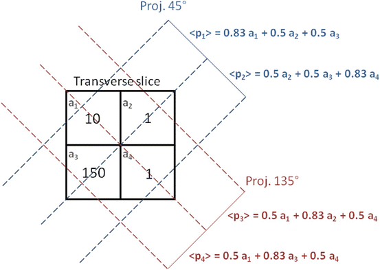

Fig. 8.3
Schematic setup in the transverse plane of a simple ideal emission 2 × 2 tomography with projections acquired at 45 and 135°. The numbers in the cells represent the mean counts emitted in the transverse slice voxels during a projection acquisition time. The symbols a i and p i are the compact labels of slice voxels and projection pixels commonly used in literature
Typically the voxel a 1 corresponds to a tumor located close to a filled bladder modelled by the voxel a 3, the voxels a 2 and a 4 modelling some residual vascular activity. In the following computations, the reader should be attentive to the difference between p i , i.e. the projection value obtained in one specific acquisition, and 〈p i 〉, i.e. the mean projection value obtained by repeating many times the acquisition under identical conditions.
This tomography acquisition setup can be simply written as a matrix product:

where the matrix c is:

giving the mean projection pixels values:
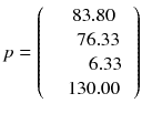
As the determinant of this matrix is non-null, the linear equation system (8.4) has a unique solution (note that using 0 and 90° in place of 45 and 135° is a degenerate case and results in a null determinant). The inverse of the matrix c can be directly computed using the minors and cofactors technique (function minverse in Excel) which gives:

A straightforward computation (mmult in Excel) shows that our example satisfies the relation:

In other words, the reconstruction of the tomographic acquisition can be performed by computing the inverse of the matrix c and making the product of this inverse with the projection.

(8.4)

(8.5)

(8.6)

(8.7)

(8.8)
Even for a SPECT using a 64 by 64 transverse voxels reconstruction, the dimension of the matrix c is already 4096 × 4096. Direct inversion of such a matrix, even with the most powerful computer, is not compatible with clinical routine (note that in order to correct the attenuation of the gamma rays in the patient, the matrix c is in reality dependent on the patient and its inversion cannot thus be computed once for all; see next section).
Fortunately, the matrix c describing an ideal tomography, i.e. where the projection pixel values come from a single LOR (perfect collimator resolution and no Compton scattering), has special properties resulting from the fact that the voxel integrations are performed along parallel LOR rotating around the slice. Using the Fourier transform theory, it is possible to prove that, for large dimensions (>16 × 16), the analytical computation (8.8) of a i can be approached by two simple steps: a RAMP filtering of the projections followed by the multiplication with the transpose of the matrix c. This second operation is commonly called “back-projection”, and the whole reconstruction called filtered back-projection (FBP). The RAMP filtering can be simply performed by multiplying the Fourier transform of the projection by the module of the spatial frequency, and the transpose c T of the matrix c is just the matrix obtained by swapping of the indices, i.e.:

In a real acquisition, the mean values 〈p i 〉 will never be observed as being inevitably corrupted by Poisson noise of magnitude  . Consider the following tomography typical acquisition values:
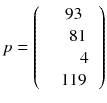
p was obtained by adding a random Poisson noise to (8.6).

(8.9)
 . Consider the following tomography typical acquisition values:
(8.10)
The computation of (8.8) using p instead of 〈p〉 gives:

We can see that a small perturbation on the projection (±10) induced a larger variation in the reconstructed voxels (±40) illustrating the ill-posedness of emission tomography; see [20] for a mathematical description. As a result the tumor, modelled by the voxel a 1, is completely obscured by the streak artefact induced by the voxel a 3 modelling the filled bladder.

(8.11)
8.2.5 Iterative EM-ML Algorithm
A more powerful reconstruction technique can be implemented after noting that the disturbing streak artefact in (8.11) contains negative voxels which do not represent a physical emission. Rather than computing the exact solution of equation (8.4), it is preferable to compute the optimal solution containing only positive voxels. By optimal solution we mean the counts distribution a j that minimizes the weighted chi-square between the acquired projections p and the projections that the distribution a i should have produced, i.e.:

where n is the reconstruction matrix size. The weighting 1/p i takes into account the corruption of the data by Poisson noise. Equation (8.12) is usually called the objective function to be optimized. Up to now, there is no existing analytical method minimizing Eq. (8.12) with  . However in our simple tomography setup (n = 2), this non-negative solution can easily be computed using the solver facility of Excel (based on the iterative Newton–Raphson algorithm) and constrained to non-negative solution. One gets:

In this case the streak artefact is almost fully removed and the voxel value a 1 modelling the tumor is partially retrieved. There are numerous and fast iterative algorithms that minimize the chi-square (8.12), such as the conjugated gradient, the Levenberg–Marquardt and the Landweber [75]. However, constraining thousands of unknowns to be non-negative during the iterations dramatically hampers the convergence speed and stability of those algorithms.

(8.12)
 . However in our simple tomography setup (n = 2), this non-negative solution can easily be computed using the solver facility of Excel (based on the iterative Newton–Raphson algorithm) and constrained to non-negative solution. One gets:
(8.13)
An alternative of minimizing the weighted chi-square is to maximize the likelihood of the solution a i . When the acquired data p i are distributed as independent Poisson variables around the mean values 〈p i 〉, it can be shown that the log of the likelihood is:

An algorithm that at each iteration step increases the likelihood (8.14) was developed [88]. This algorithm always converges because there exists an upper bound value for the likelihood (8.14). This algorithm called expectation maximization of the maximum likelihood (EM-ML) is:

Usually, the initial solution is chosen to be  for all i. As all the c ij are non-negative, this choice of initial solution preserves in a natural way the non-negativity of the solution. In our 2 × 2 example, Eq. (8.15) converges to:

Note that EM-ML is a multiplicative algorithm and is thus non-linear, i.e. the sum of the reconstruction of two acquisitions is not equal to the reconstruction of the sum of the two acquisitions, i.e.:

The right-hand side scenario provides the best result.

(8.14)

(8.15)
 for all i. As all the c ij are non-negative, this choice of initial solution preserves in a natural way the non-negativity of the solution. In our 2 × 2 example, Eq. (8.15) converges to:
(8.16)

(8.17)
The EM-ML also has the drawback to have a very slow and non-uniform convergence speed: hundreds or even thousands of iterations are needed to come close to the solution, especially in the low count regions (Fig. 8.4).
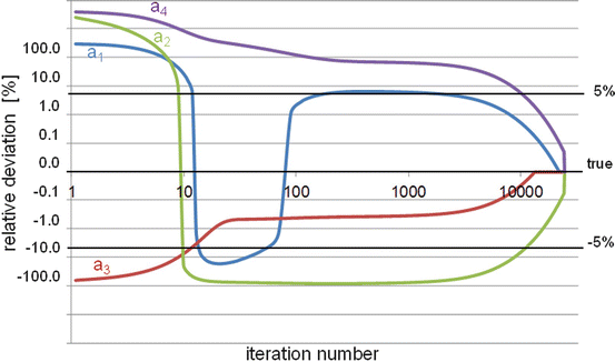

Fig. 8.4
Pseudo-log-log representation of the relative deviation (RD) as a function of the EM-ML iteration number. Although only about 11 iterations are needed to get an RD better than 5 % for the voxel a 3 (value = 150), more than 2000 and 10,000 iterations are needed for the voxel a 1 (value = 10) and the voxels a 2 and a 4 (value = 1) to get the same accuracy, respectively
8.2.6 FBP, EM-ML and OSEM in Clinical Studies
To reduce the computation time, an accelerated version of EM-ML called ordered subset expectation maximization (OSEM) was developed [38] and became the standard algorithm in tomographic reconstruction. Boost speed factor of about 30 can be reached; however OSEM does not overcome the non-uniform convergence speed issue.
Physically, c ij represents the probability that a photon emitted in the voxel a j will be detected in the pixel p i . When physical effects such as non-uniform attenuation, Compton scattering and detector response are included in the modelling of this probability c ij , it is no longer possible to reconstruct the tomography using analytical methods such as FBP. On the other hand, iterative algorithms like EM-ML (Eq. 8.15) naturally compensate these disturbing physical effects during the reconstruction. This further explains why since a decade EM-ML or OSEM have superseded the historical FBP reconstruction in most SPECT and PET routines.
Figure 8.5 shows reconstructions of a phantom modelling, a typical 111In-octreotate SPECT study. Conventional FBP reconstruction using a Shepp–Logan filter does not allow visualizing the two modelled tumors that are overshadowed by the streak artefact originating by the active kidney cortices. The EM-ML reconstruction clearly reveals the presence of the modelled tumors. Note also the better cortex delineation and contrast with the kidney pelvis as a result of the inclusion of the Compton scattering and of the collimator response in the EM-ML algorithm.
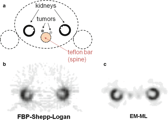

Fig. 8.5
(a) Drawing in the transverse plane of the phantom modelling, a typical 111In-octreotate study, all compartments are filled with water, besides a Teflon bar modelling the spine attenuation. Specific 111In concentrations in the two tumors were 50 and 25 % that of the modelled kidney cortex. (b, c): SPECT 30 min acquisition of the phantom performed on a Trionix Triad XLT20 camera equipped with a MEGP collimator and reconstructed in matrix 64 × 64 with FBP (b) and EM-ML (c), respectively. Compton scattering [114] and collimator PSF were included in the EM-ML reconstruction. Note the clear visualization of the modelled tumors in the EM-ML reconstruction, while in FBP they are overshadowed by the streak artefact originating from the kidneys
In contrary, most CT studies are still reconstructed with FBP. This results from two major features. First, CT scan requires reconstruction matrix size much larger than in SPECT or PET which dramatically increases the reconstruction time when using EM-ML-based algorithms. Secondly, as the dose is delivered to the patient only during the acquisition time, and not during several hours such as in SPECT and PET, CT can benefit from higher acquisition counting rates. This reduces the noise present in the acquired data and the need to use EM-ML-based algorithms. However, due to the endless increasing concern about patient radioprotection, all CT manufacturers are now proposing iterative reconstruction algorithm with their systems in order to reduce the patient irradiation [8, 39, 70, 71].
8.2.7 EM-ML and OSEM Regularization
Although the non-negativity of EM-ML well overcomes the streak artefact issues in low count region, EM-ML does not succeed as well in large count regions where the ill-posed nature of tomography induces high negative–positive fluctuations around the actual counts. The amplitude and the frequency of these fluctuations increase with the number of iterations. A simple method to address this issue is to limit the number of iterations, which in some way regularizes the problem. However, due to the non-uniform convergence speed, this approach cannot be recommended when the target tissue is located close to a more active tissue, which is often the case in nuclear medicine.
A popular way to regularize the problem is to add some penalty function P to the likelihood and to maximize the cost function:

The goal is now to find the solution a j that maximizes Q(a). The penalty function P(a) is constructed such that P(a) increases with fluctuations in a i . In other words, the first term in (8.18) penalizes solutions which do not fit well the acquired data, while the second penalizes solutions containing unphysical variations. Note that Eq. (8.18) contains an adjustable parameter λ. A very simple penalty function is:

It is very simple to check that for a constant total count  , the solution that maximizes −P(a) is the uniform solution
  , i.e. the smoothest solution (e.g. if n = 2 and C = 8,
 ![$$ {5}^2+{3}^2 > {4}^2+{4}^2) $$
” src=”http://oncohemakey.com/wp-content/uploads/2017/10/A339179_1_En_8_Chapter_IEq9.gif”></SPAN>. Obviously, this simple penalty function has the drawback to also smooth the actual activity transition at the tissue boundaries.</DIV><br />
<DIV id=Par32 class=Para>There is a very abundant literature about regularization methods [<CITE><A href=]() 10, 20, 24, 62–64]. Popular regularization methods are:
10, 20, 24, 62–64]. Popular regularization methods are:

(8.18)

(8.19)
 , the solution that maximizes −P(a) is the uniform solution
  , i.e. the smoothest solution (e.g. if n = 2 and C = 8,
The use of various sophisticated penalty functions or Bayesian prior designed to better preserve the actual edge transitions, such as the promising total variation method [14].
Blob-based reconstruction, where the reconstruction is not performed on adjacent voxels but on overlapping voxels (called blobs) of various shapes and diameters playing the role of regularization parameter λ. The inter-blobs coupling due to the overlapping stabilizes the reconstruction and avoids excessive fluctuations.
Combinations of these different regularization methods are also proposed. Once in a while, one manufacturer claims to have succeeded in implementing the ultimate reconstruction algorithm that provides a noise-free image without any compromising of the resolution, giving self-important and attractive name to their reconstruction software. The reality is that despite intense works performed by mathematicians during the last two decades, this ideal regularization has not yet been found. Current regularizations still include some trade-off between noise reduction and resolution smoothing through the regularization parameter λ which in practice depends in an obscure way on the acquired data. Manufacturers continuously improve empirical relations giving the regularization parameter as a function of the tracers used, tissue studied and patient size. All these considerations advise the clinician to pay attention to the image rendering.
8.2.8 Conditioning Improvement in Emission Tomography
Although during 40 years the ill-posed nature of emission tomography was only addressed in the reconstruction process and only intensively for the last two decades, a major breakthrough was initiated in 2006 with the launching of the first successful commercial time-of-flight (TOF) PET system [102]. Indeed, by measuring the arrival delay between the two 511 keV γ-rays on the detector ring, it is possible to get information about the decay location on the LOR. Current TOF-PET systems have a TOF resolution of about 320 ps [101] which corresponds to a spatial resolution of about 5 cm on the decay location on the LOR. Using such a system, two decays occurring at two positions –t and t on the LORs (see Fig. 8.2a) more than 5 cm apart will be counted in two different TOF projections. As a result negative and positive offset around the actual counts will no longer cancel each other. In other words, the distribution (8.1) is now a visible object for a TOF-PET system, and only the distribution (8.1) truncated inside the radius r = 2.5 cm will remain an invisible object. TOF information really reduces the ill-posed nature of the tomography acquisition [4, 18] rather than lowering its impact on the reconstructed data. As a result TOF significantly reduces noise artefact (Fig. 8.6), especially in corpulent patient where the higher attenuation reduces the count rate and thus increases the noise in acquired data [50].


Fig. 8.6
Reduction of the artefacts present around the bladder in non-TOF reconstruction (Courtesy of Dr. Joel Karp)
Since a decade an intense race is engaged between physics labs in order to reach a TOF resolution of 25 ps corresponding to a decay localisation resolution of 4 mm [111]. When reached, this TOF resolution will allow the direct positioning of the decay in the appropriate 4 mm transverse voxel without any reconstruction process: TOF-PET will become a full well-posed problem. In consequence, all the noise artefacts will disappear; noise will no longer be correlated in the transverse slice and will follow the Poisson distribution such as in planar view. From 2006 to 2015, the TOF resolution of commercial systems improved from 650 ps to 320 ps [60, 101, 103]. In physics labs, TOF resolution of 75 ps was reached, but using a simple two-arm detectors equipped with pure thin CsBr crystal [89].
A similar breakthrough for SPECT is in preparation in physics labs with the development of recoil electron-tracking Compton camera using pressurized gas chamber [46, 47]. With this camera, the LOR of the decay is determined without the use of a collimator. Surrounding the patient with such cameras and using multi γ-rays emitters, such as 111In, 67Ga or 95Tc, the decay location will directly be obtained without any reconstruction process [111].
8.3 CT
8.3.1 Principles
In CT, an anatomical image is derived from the total attenuation underwent by x-rays along different angles around the patient. The radiation intensity reaching the detector is given by

where I 0 is the source intensity, μ(x,y) is the patient attenuation coefficient and R θ is the rotation by an angle θ. Taking the logarithm gives:

Projections p are the sum of the attenuation coefficients along the LORs and can thus be reconstructed in the same way that emission tomography where the projections are the sum of the activity. For a specific photon energy, regarding that mammalians are mainly made of low atomic number Z elements (Z ≤ 8), the attenuation coefficient mainly depends on the crossed tissues density.

(8.20)

(8.21)
CT reconstructed images are usually displayed in Hounsfield units, defined as

where μ w is the attenuation coefficient of water at the x-ray beam energy used.

(8.22)
Clinical CT developed in [36] is still in continuous improvement [22, 48]. The first CT generation was composed of only one x-ray source and one detector cell translating and rotating together around the patient (Fig. 8.7a). Next, the number of detector cells was increased in order to reduce the acquisition time (Fig. 8.7b). Most current CT scanners are from the third generation where an x-ray fan beam is detected by many cells forming an arc or a flat panel [29, 30] (Fig. 8.7c). In some systems, the source-detector couple rotates around the patient while the patient table translates, resulting in a helical acquisition, often called spiral. There exists a fourth generation of CT scanner where the detector is a full stationary ring around the patient (Fig. 8.7d).
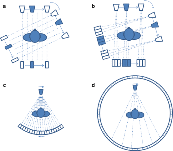

Fig. 8.7
Four generations of CT scan. (a, b) First and second generation: one beam source and detector(s) couple translating and rotating around the patient. (c) Third generation: fan beam source and arc-shaped detector couple rotating around the patient. (d) Fourth generation: fan beam source rotating around the patient surrounded by a full-ring static detector
Note that similarly to PET, no mechanical collimation is needed, the LOR being the line going from the x-ray point source to the detector cell reached.
The development of fast spiral CT scanner in the 1980s gave a boost to the use of CT in medical imaging. Shorter scans make it possible for patients to hold their breath during the scan which reduces motion artefacts. Spiral CT scans are characterized by the pitch factor, equal to the ratio of the distance covered by the table in one source revolution over the detector axial width (or slice thickness). In practice the pitch factor is chosen between 1 and 1.8. A higher pitch corresponds to faster volume coverage, but also to fewer data samples as the gap between samples increases [37]. Note that with the introduction of multi-row detector, some controversies and discrepancies appeared in the definition of the pitch [91].
8.3.2 Beam-Hardening Artefacts
Beam-hardening artefacts are due to the non-monochromatic nature of the x-ray beam source which is produced by fast electrons colliding with a solid metal anode. This generates a continuous energy spectrum up to a maximum energy fixed by the high voltage applied between the cathode and anode, i.e. the “kV” value. When travelling into the patient’s body, the low-energy part of the spectrum is more attenuated making the beam harder and harder. As a result, the beam is less and less attenuated by the tissue, resulting in an underestimation of the tissue density in the reconstruction image (Fig. 8.8).


Fig. 8.8
(a) Beam-hardening artefact due to the stronger attenuation of bone tissues (Reprinted from [27] with permission of the society of nuclear medicine). (b) Schematic explanation. a: Typical CT energy spectrum. b and c: Hardened energy spectra after crossing 5 cm of bone and water, respectively. d and e: Resulting energy spectra after crossing an additional 5 cm of water. Due to the higher hardening by bone, the ratio of the total counts between spectra d and b (i.e. 0.37 = 40/108) corresponds to a pseudo less attenuating additional tissue than the one exhibited by the ratio of spectra e and c (i.e. 0.34 = 107/313)
A simple correction, implemented in all modern CT scanner to reduce the beam-hardening artefacts, consists in adding an aluminium or copper plate between the source and the patient to filter the low energetic photons.
The beam-hardening of the x-ray spectrum also induces errors in the reconstructed image in the form of under-evaluated attenuation coefficients in the central region of the patient. These are called cupping artefacts. Most CT scanners include software corrections for these artefacts based on a calibration of the system with a water phantom. Of course these corrections are not adapted for bone tissues as these attenuate the x-ray beam a lot more than water or soft tissues. In that case more sophisticated techniques are needed to correct for beam-hardening artefacts. One solution is to combine CT scans acquired with two different energies, i.e. two different maximum high voltages [44]. By combining the projections obtained with the two scans, it is possible to reconstruct the image without beam-hardening artefacts [15].
Stay updated, free articles. Join our Telegram channel

Full access? Get Clinical Tree


