Guide to Clinical Studies

Eitan Amir and Ian F. Tannock

22.1 INTRODUCTION

To select the optimal treatment for patients, clinical oncologists need to be skilled at critically evaluating data from clinical studies and interpreting these appropriately. Clinicians should also be proficient in the application of diagnostic tests, assessment of risk, and the estimation of prognosis. Equally, scientists involved in translational research should be aware of the problems and pitfalls in undertaking clinical studies. This chapter provides a critical overview of methods used in clinical research.

22.2 TREATMENT

22.2.1 Purpose of Clinical Trials

Clinical trials are used to assess the effects of specific interventions on the health of individuals. Possible interventions include treatment with drugs, radiation, or surgery; modification of diet, behavior, or environment; and surveillance with physical examination, blood tests, or imaging tests. This section focuses on trials of treatment.

Clinical trials may be separated conceptually into explanatory trials, designed to evaluate the biological effects of treatment, and pragmatic trials, designed to evaluate the practical effects of treatment (Schwartz et al, 1980). This distinction is crucial, because treatments that have desirable biological effects (eg, the ability to kill cancer cells and cause tumor shrinkage) may not have desirable effects in practice (ie, may not lead to improvement in duration or quality of life). Table 22–1 lists the major differences between explanatory and pragmatic trials.

TABLE 22–1 Classification of clinical trials.

The evaluation of new cancer treatments usually involves progression through a series of clinical trials. Phase I trials are designed to evaluate the relationship between dose and toxicity and aim to establish a tolerable schedule of administration. Phase II trials are designed to screen treatments for their antitumor effects in order to identify those worthy of further evaluation. Phase I and Phase II trials are explanatory—they assess the biological effects of treatment on host and tumor in small numbers of subjects to guide decisions about further research. Randomized Phase III trials are designed to determine the usefulness of new treatments in the management of patients, and are therefore pragmatic. Randomization is the process of assigning participants to experimental and control (existing) therapy, with each participant having a pre-specified (usually equal) chance of being assigned to any group.

Phase I trials are used commonly to define the maximum tolerable dose of a new drug, with a focus on the relationship between dosage and toxicity and on pharmacokinetics (see Chap. 18, Sec. 18.1). Small numbers of patients are treated at successively higher doses until the maximum acceptable degree of toxicity is reached. Many variations have been used; a typical design is to use a low initial dose, unlikely to cause severe side effects, based on tolerance in animals. A modified Fibonacci sequence is then used to determine dose escalations: Using this method, the second dose level is 100% higher than the first, the third is 67% higher than the second, the fourth is 50% higher than the third, the fifth is 40% higher than the fourth, and all subsequent levels are 33% higher than the preceding levels. Three patients are treated at each level until any potentially dose-limiting toxicity is observed. Six patients are treated at any dose where such dose-limiting toxicity is encountered. The maximum tolerated dose (MTD) is defined as the maximum dose at which dose-limiting toxicity occurs in fewer than one-third of the patients tested. This design is based on experience that few patients have life-threatening toxicity and on the assumption that the MTD is also the most effective anticancer dose. It has been criticized because most patients receive doses that are well below the MTD and are therefore participating in a study where they have little chance of therapeutic response. Adaptive trials using accelerated titration where fewer patients are treated at the lowest doses, and Bayesian dose-finding designs where the magnitude of dose increments is determined by toxicity observed at lower doses, have been suggested as methods to address this limitation (Simon et al, 1997; Yin et al, 2006). Furthermore, it has been suggested that for molecular-targeted agents, use of MTD is less meaningful. First, MTD generally defines acute toxicity. The use of targeted agents is usually chronic and chronic tolerability is often independent of acute tolerability. Second, early clinical trials of biological agents demonstrated that maximal beneficial effects could be seen at doses lower than the MTD. This led to the concept of the optimal biological dose, which is defined as the dose that produces the maximal beneficial effects with the fewest adverse events (Herberman, 1985). However, difficulties in determination of the optimal biological dose mean that it only rarely forms the basis of dose selection of targeted agents (Parulekar and Eisenhauer, 2004).

Phase II trials are designed to determine whether a new treatment has sufficient anticancer activity to justify further evaluation, although particularly when evaluating targeted agents, they should ideally provide some information about target inhibition and, hence, mechanism of action. They usually include highly selected patients with a given type of cancer and may use a molecular biomarker to define patients most likely to respond (eg, expression of the estrogen receptor in women with breast cancer when evaluating a hormonal agent; see Chap. 20, Sec. 20.4.1). Phase II studies usually exclude patients with “nonevaluable” disease, and use the proportion of patients whose tumors shrink or disappear (response rate) as the primary measure of outcome. Their sample size is calculated to distinguish active from inactive therapies according to whether response rate is greater or less than some arbitrary or historical level. The resulting sample size is inadequate to provide a precise estimate of activity. For example, a Phase II trial with 24 patients and an observed response rate of 33% has a 95% confidence interval of 16% to 55%. Tumor response rate is a reasonable end point for assessing the anticancer activity of a cytotoxic drug and can predict for eventual success of a randomized Phase III trial. However, response rate is a suboptimal end point in trials evaluating targeted agents, which can modify time to tumor progression without causing major tumor shrinkage (El-Maraghi and Eisenhauer, 2008). Furthermore, it is not a definitive measure of patient benefit. Phase II trials are suitable for guiding decisions about further research but are rarely suitable for making decisions about patient management. There are 2 dominant designs to Phase II trials: single-arm and randomized. Single-arm Phase II trials are simple, easy to execute, and require small sample sizes. They are also able to restrict false-positive and false-negative rates to reasonable levels. However, results usually need to be compared to historical controls. In contrast, randomized Phase II designs are more complex, require up to 4-fold more patients as compared with single-arm trials, but do provide more robust preliminary evidence of comparative efficacy. Single-arm trials may be preferred for single agents with tumor response end points. They may also be preferable in less common tumor sites where accrual may be more challenging. Randomized designs may be favorable for trials of combination therapy and with time to event end points (Gan et al, 2010). The literature is confusing, however, because Phase II trials, especially those with randomized designs have sometimes been reported and interpreted as if they did provide definitive answers to questions about patient management.

Phase III trials are designed to answer questions about the usefulness of treatments in patient management. Questions about patient management are usually comparative, as they involve choices between alternatives—that is, an experimental versus the current standard of management. The current standard may include other anticancer treatments or may be “best supportive care” without specific anticancer therapy. The aim of a Phase III trial is to estimate the difference in outcome associated with a difference in treatment, sometimes referred to as the treatment effect. Ideally, alternative treatments are compared by administering them to groups of patients that are equivalent in all other respects, that is, by randomization of suitable patients between the current standard and the new experimental treatment. Randomized controlled Phase III trials are currently regarded as the best, and often only, reliable means of determining the usefulness of treatments in patient management. Phase III drug trials are often conducted in order to register drug treatment for particular indications, which requires approval by agencies such as the United States Food and Drug Administration (FDA) or the European Medicines Agency (EMA). Their end points should reflect patient benefit, such as duration and quality of survival. Most randomized Phase III clinical studies are designed to show (or exclude) statistically significant improvements in overall survival, although many cancer trials use surrogate end points such as disease-free survival (DFS) or progression-free survival (PFS) as the primary end point. The use of a surrogate end point is only clinically meaningful if it has been validated as predicting for improvement in overall survival or quality of life (see below). The following discussion focuses on randomized controlled Phase III trials.

One criticism of the structure of clinical trials is that it takes a long time for drugs to go from initial (Phase I) testing to regulatory approval (based on results of Phase III trials). More recently, more adaptive designs have been introduced to try to speed up drug development. The multiarm, multistage trial design (Royston et al, 2003) is a new approach for conducting randomized trials. It allows several agents or combinations of agents to be assessed simultaneously against a single control group in a randomized design. Recruitment to research arms that do not show sufficient promise in terms of an intermediate outcome measure may be discontinued at interim analyses. In contrast, recruitment to the control arm and to promising research arms continues until sufficient numbers of patients have been entered to assess the impact in terms of the definitive primary outcome measure. By assessing several treatments in one trial, this design allows the efficacy of drugs to be tested more quickly and with smaller numbers of patients compared with a program of separate Phase II and Phase III trials.

Another criticism is that in an era of molecular-targeted therapy, treatments are often provided on an empirical basis with few trials assessing novel methods for enriching participants for those most likely to benefit from the experimental therapy. Trials with biomarkers selecting patients for benefit have needed smaller sample size to detect similar levels of benefit to those not using biomarkers to select a probable drug-sensitive population (Amir et al, 2011). Some agents (eg, imatinib for the treatment of patients with gastrointestinal stromal tumors [GISTs]) did not need randomized Phase III trials to detect substantial benefits. There are 2 broad ways to select patients for targeted drugs based on biomarkers. In the enrichment approach, all patients are assessed prospectively for presence of the biomarker, and only those with the bio-marker are included in the trial (eg, trastuzumab in human epidermal growth receptor 2 [HER2]-positive breast cancer). In the retrospective approach the presence or absence of a biomarker is determined in all treated patients and related to the probability of response to a targeted agent (eg, panitumumab in colorectal cancer in relation to K-ras mutations). The enrichment approach leads to greater economic value across the drug development pathway and could reduce both the time and costs of the development process (Trusheim et al, 2011).

22.2.2 Sources of Bias in Clinical Trials

Important characteristics of the patients enrolled in a clinical trial include demographic data (eg, age and gender), clinical characteristics (the stage and pathological type of disease), general well-being, and activities of daily life (performance status), as well as other prognostic factors. Phase III trials are most likely to have positive outcomes if they are applied to homogenous populations. Consequently, most usually have multiple exclusion criteria, such that patients with selected comorbidities and use of some concomitant medications are often excluded. For this and other unknown reasons, patients enrolled in clinical trials often have better outcomes (even if receiving standard treatment) than patients who are seen in routine practice (Chua and Clarke, 2010). The selection of subjects and inclusion and exclusion criteria must be described in sufficient detail for clinicians to judge the degree of similarity between the patients in a trial and the patients in their practice. Treatments, whether with drugs, radiation, or surgery, must be described in sufficient detail to be replicated. Because not all patients may receive the treatment as defined in the protocol, differences between the treatment specified in the protocol and the treatment actually received by the patients should be reported clearly. Although patients in randomized trials may differ from those seen in clinical practice, this difference does not usually detract from the primary conclusion of a randomized trial, although the selection of patients may limit the ability to generalize results to an unselected population.

Treatment outcomes for patients with cancer often depend as much on their initial prognostic characteristics as on their subsequent treatment, and imbalances in prognostic factors can have profound effects on the results of a trial. The reports of most randomized clinical trials include a table of baseline prognostic characteristics for patients assigned to each arm. The p-values often reported in these tables are misleading, as any differences between the groups, other than the treatment assigned, are known to have arisen by chance. The important question as to whether any such imbalances influence the estimate of treatment effect is best answered by an analysis that is adjusted for any imbalance in prognostic factors (see Sec. 22.4).

Compliance refers to the extent to which a treatment is delivered as intended. It depends on the willingness of physicians to prescribe treatment as specified in the protocol and the willingness of patients to take treatment as prescribed by the physician. Patient compliance with oral medication is variable and may be a major barrier to the delivery of efficacious treatments (Hershman et al, 2010).

Contamination occurs when people in one arm of a trial receive the treatment intended for those in another arm of the trial. This may occur if people allocated to placebo obtain active drug from elsewhere, as has occurred in trials of treatments for HIV infection. This type of contamination is rare in trials of anticancer drugs but common in trials of dietary treatments, vitamin supplements, or other widely available agents. The effect of contamination is to blur distinctions between treatment arms.

Crossover is a related problem that influences the interpretation of trials assessing survival duration. It occurs when people allocated to one treatment subsequently receive the alternative treatment when their disease progresses. Although defensible from pragmatic and ethical viewpoints, crossover changes the nature of the question being asked about survival duration. In a 2-arm trial without crossover, the comparison is of treatment A versus treatment B, whereas with crossover, the comparison is of treatment A followed by treatment B versus treatment B followed by treatment A.

Cointervention occurs when treatments are administered that may influence outcome but are not specified in the trial protocol. Examples are blood products and antibiotics in drug trials for acute leukemia, or radiation therapy in trials of systemic adjuvant therapy for breast cancer. Because cointerventions are not allocated randomly, they may be distributed unequally between the groups being compared and can contribute to differences in outcome.

22.2.3 Importance of Randomization

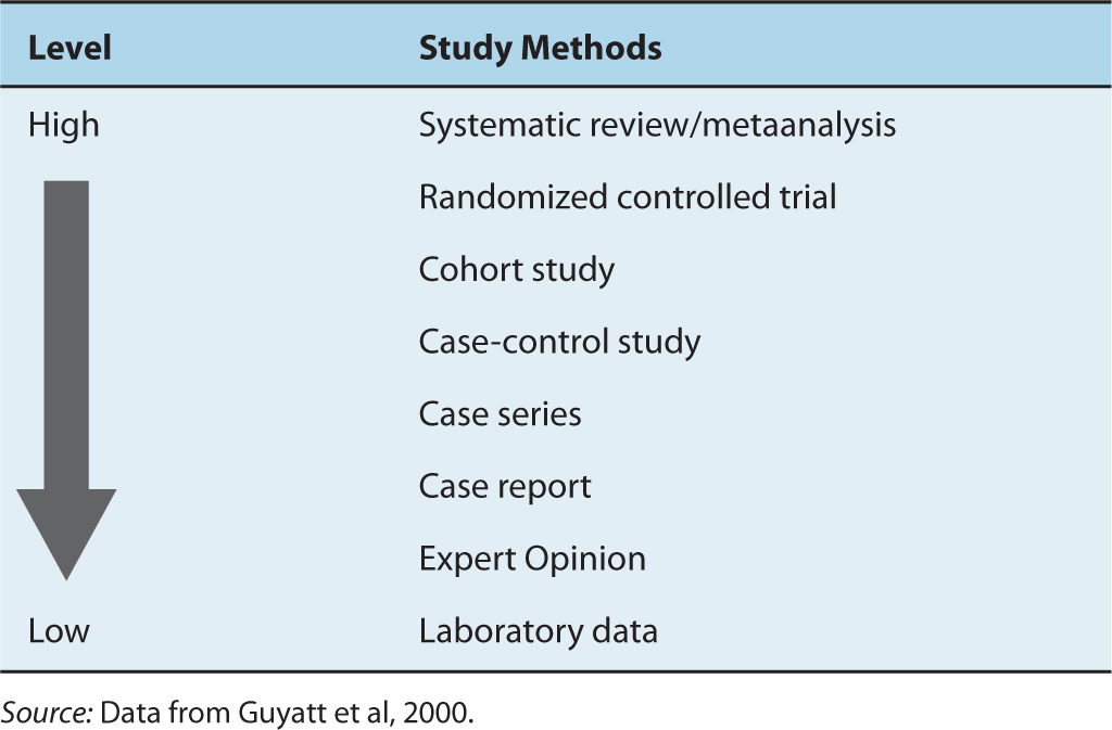
Well-conducted randomized trials provide a high level of evidence about the value of a new treatment (Table 22–2). The ideal comparison of treatments comes from observing their effects in groups that are otherwise equivalent, and randomization is the only effective means of achieving this. Comparisons between historical controls, between concurrent but nonrandomized controls, or between groups that are allocated to different treatments by clinical judgment, are almost certain to generate groups that differ systematically in their baseline prognostic characteristics. Important factors that are measurable can be accounted for in the analysis; however, important factors that are poorly specified—such as comorbidity, a history of complications with other treatments, the ability to comply with treatment, or family history—cannot. Comparisons based on historical controls are particularly prone to bias because of changes over time in factors other than treatment, including altered referral patterns, different criteria for selection of patients, and improvements in supportive care. These changes over time are difficult to assess and difficult to adjust for in analysis. Such differences tend to favor the most recently treated group and to exaggerate the apparent benefits of new treatments.

TABLE 22–2 Hierarchy of evidence.

Stage migration causes systematic variation (Fig. 22–1), and occurs when patients are assigned to different clinical stages because of differences in the precision of staging rather than differences in the true extent of disease. This can occur if patients staged very thoroughly as part of a research protocol are compared with patients staged less thoroughly in the course of routine clinical practice, or if patients staged with newer more-accurate tests are compared with historical controls staged with older, less-accurate tests. Stage migration is important because the introduction of new and more sensitive diagnostic tests produces apparent improvements in outcome for each anatomically defined category of disease in the absence of any real improvement in outcome for the disease overall (Feinstein et al, 1985). This paradox arises because, in general, the patients with the worst prognosis in each category are reclassified as having more advanced disease. As illustrated in Figure 22–1, a portion of those patients initially classified as having localized disease (stage I) may be found to have regional spread if more sensitive imaging is used, and a portion of those initially classified as having only regional spread (stage II) will be found to have systemic spread (stage III). With more-sensitive testing, fewer patients classified as having localized disease will actually have regional spread, making the measured outcome of the localized group appear improved. Similarly, the outcome of patients newly classified as having regional disease will be better than that of those with larger volumes of regional disease seen on less-sensitive tests, thereby improving the outcomes of the regional disease group. The same applies for patients moving from the regional to the systemic category. As a consequence, the prognosis of each category of disease improves in the absence of any real improvement in the prognosis of the disease overall.

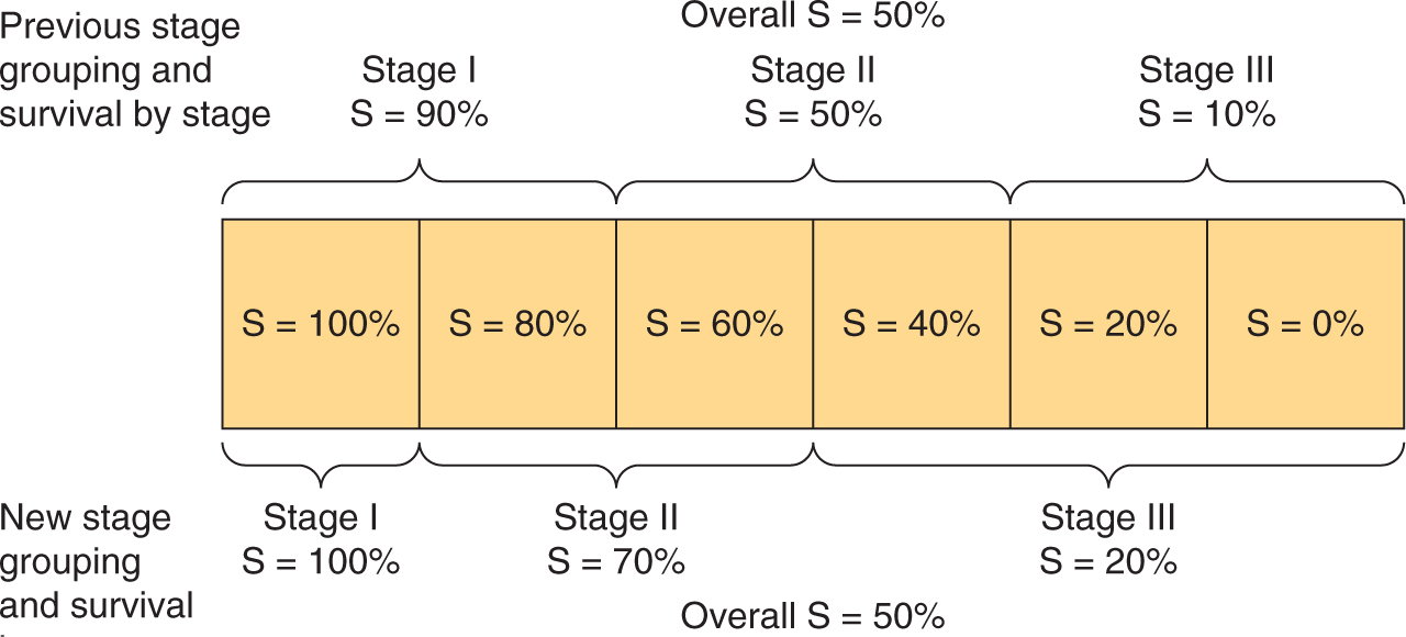
FIGURE 22–1 Stage migration. The diagram illustrates that a change in staging investigations may lead to the apparent improvement of results within each stage without changing the overall results. In the hypothetical example, patients are divided into 6 equal groups, each with the indicated survival. Introduction of more-sensitive staging investigations moves patients into higher-stage groups, as shown, but the overall survival of 50% remains unchanged. (Adapted from Bush, 1979.)

The major benefit of randomization is the unbiased distribution of unknown and unmeasured prognostic factors between treatment groups. However, it is only ethical to allocate patients to treatments randomly when there is uncertainty about which treatment is best. The difficulty for clinicians is that this uncertainty, known as equipoise, usually resides among physicians collectively rather than within them individually.

Random allocation of treatment does not ensure that the treatment groups are equivalent, but it does ensure that any differences in baseline characteristics are a result of chance. Consequently, differences in outcome must be a result of either chance or treatment. Standard statistical tests estimate the probability (p value) that differences in outcome, as observed, might be a result of chance alone. The lower the p value, the less plausible is the null hypothesis that the observed difference is a result of chance, and the more plausible is the alternate hypothesis that the difference is a result of treatment.

Imbalances in known prognostic factors can be reduced or avoided by stratifying and blocking groups of patients with similar prognostic characteristics during the randomization procedure. For example, in a trial of adjuvant hormone therapy for breast cancer, patients might be stratified according to the presence or absence of lymph node involvement, hormone receptor levels, and menopausal status. Blocking ensures that treatment allocation is balanced for every few patients within each defined group (strata). This is practical only for a small number of strata. Randomization in multicenter trials is often blocked and stratified by treatment center to account for differences between centers; however, this carries the risk that when there is almost complete accrual within a block the physicians may know the arm to which the next patient(s) will be assigned, creating the possibility of selection bias (see below). An alternative approach to adjust for imbalances in prognostic factors is to use multivariable statistical methods (see Sec. 22.4.1 and Chap. 3, Sec 3.3.3).

For randomization to be successfully implemented and to reduce bias, the randomization sequence must be adequately concealed so that the investigators, involved health care providers, and subjects are not aware of the upcoming assignment. The absence of adequate allocation concealment can lead to selection bias, one of the very problems that randomization is supposed to eliminate. Historically, allocation concealment was achieved by the use of opaque envelopes, but in multicenter studies, centralized or remote telephone-based, computer-based, or internet-based allocation systems are now used.

If feasible, it is preferable that both physicians and patients be unaware of which treatment is being administered. This optimal double-blind design prevents bias. Evidence for bias in nonblinded randomized trials comes from the observation that they lead more often to apparent improvements in outcome from experimental treatment than blinded trials and that assignment sequences in randomized trials have sometimes been deciphered (Chalmers et al, 1983; Wood et al, 2008).

22.2.4 Choice and Assessment of Outcomes

The measures used to assess a treatment should reflect the goals of that treatment. Treatment for advanced cancer is often given with palliative intent—to prolong survival or reduce symptoms without realistic expectation of cure. Survival duration has the advantage of being an unequivocal end point that can be unambiguously measured, but if a major end point is improved quality of life, then appropriate methods should be used to measure quality of life. Anti-cancer treatments may prolong survival through toxic effects on the cancer or may shorten survival through toxic effects on the host. Similarly, anticancer treatments may improve quality of life by reducing cancer-related symptoms or may worsen quality of life by adding toxicity due to treatment. Patient benefit depends on the trade-off between these positive and negative effects, which can be assessed only by measuring duration of survival and quality of life directly.

Surrogate or indirect measures of patient benefit, such as tumor shrinkage, DFS, or PFS, can sometimes provide an early indication of efficacy, but they are not substitutes for more direct measures of patient benefit. For example, the use of DFS rather than overall survival in studies of adjuvant treatment requires fewer subjects and shorter follow-up but ignores what happens following the recurrence of disease. Surrogate measures can be used if they have been validated as predicting for benefit in clinically relevant end points such as the use of DFS as a surrogate for overall survival in patients with colorectal cancer receiving fluorouracil-based treatment (Sargent et al, 2005). Higher tumor response rates or improvements in DFS do not always translate into longer overall survival or better quality of life (Ng et al, 2008). Changes in the concentration of tumor markers in serum, such as prostate-specific antigen (PSA) for prostate cancer or cancer antigen 125 (CA125) in ovarian cancer, have been used as outcome measures in certain types of cancer. Levels of these markers may reflect tumor burden in general, but the relationship is quite variable; there are individuals with extensive disease who have low levels of a tumor marker in serum. The relationship between serum levels of a tumor marker and outcome is also variable. In men who have received local treatment for early stage prostate cancer, the reappearance of PSA in the serum indicates disease recurrence. In men with advanced prostate cancer, however, baseline levels of serum PSA may not be associated with duration of survival, and changes in PSA following treatment are not consistently related to changes in symptoms.

It is essential to assess outcomes for all patients who enter a clinical trial. It is common in cancer trials to exclude patients from the analysis on the grounds that they are “not evaluable.” Reasons for nonevaluability vary, but may include death soon after treatment was started or failure to receive the full course of treatment. It may be permissible to exclude patients from analysis in explanatory Phase II trials that are seeking to describe the biological effects of treatment; these trials indicate the effect of treatment in those who were able to complete it. It is seldom appropriate to exclude patients in randomized trials, which should reflect the conditions under which the treatment will be applied in practice. Such trials test a policy of treatment, and the appropriate analysis for a pragmatic trial is by intention to treat: patients should be included in the arm to which they were allocated regardless of their subsequent course.

For some events (eg, death) there is no doubt as to whether the event has occurred, but assignment of a particular cause of death (eg, whether it was cancer related) may be subjective, as is the assessment of tumor response, recognition of tumor recurrence, and therefore determination of DFS. The compared groups should be followed with similar types of evaluation so that they are equally susceptible to the detection of outcome events such as recurrence of disease. Whenever the assessment of an outcome is subjective, variation between observers should be examined. Variable criteria of tumor response and imprecise tumor measurement have been documented as causes of variability when this end point is used in clinical trials.

22.2.5 Survival Curves and Their Comparison

Subjects may be recruited to clinical trials over several years, and followed for an additional period to determine their time of death or other outcome measure. Subjects enrolled early in a trial are observed for a longer time than subjects enrolled later and are more likely to have died by the time the trial is analyzed. For this reason, the distribution of survival times is the preferred outcome measure for assessing the influence of treatment on survival. Survival duration is defined as the interval from some convenient “zero time,” usually the date of enrollment or randomization in a study, to the time of death of any cause. Subjects who have died provide actual observations of survival duration. Subjects who were alive at last follow-up provide censored (incomplete) observations of survival duration; their eventual survival duration will be at least as long as the time to their last follow-up. Most cancer trials are analyzed before all subjects have died, so a method of analysis, which accounts for censored observations, is required.

Actuarial survival curves provide an estimate of the eventual distribution of survival duration (when everyone has died), based on the observed survival duration of those who have died and the censored observations of those still living. Actuarial survival curves are preferred to simple cross-sectional measures of survival because they incorporate and describe all of the available information. Table 22–3 illustrates the life-table method for construction of an actuarial survival curve. The period of follow-up after treatment is divided into convenient short intervals—for example, weeks or months. The probability of dying in a particular interval is estimated by dividing the number of people who died during that interval by the number of people who were known to be alive at its beginning (E = C/B in Table 22–3). The probability of surviving a particular interval, having survived to its beginning, is the complement of the probability of dying in it (F = 1 – E). The actuarial estimate of the probability of surviving for a given time is calculated by cumulative multiplication of the probabilities of surviving each interval until that time (Fig. 22–2).

TABLE 22–3 Calculation of actuarial survival.

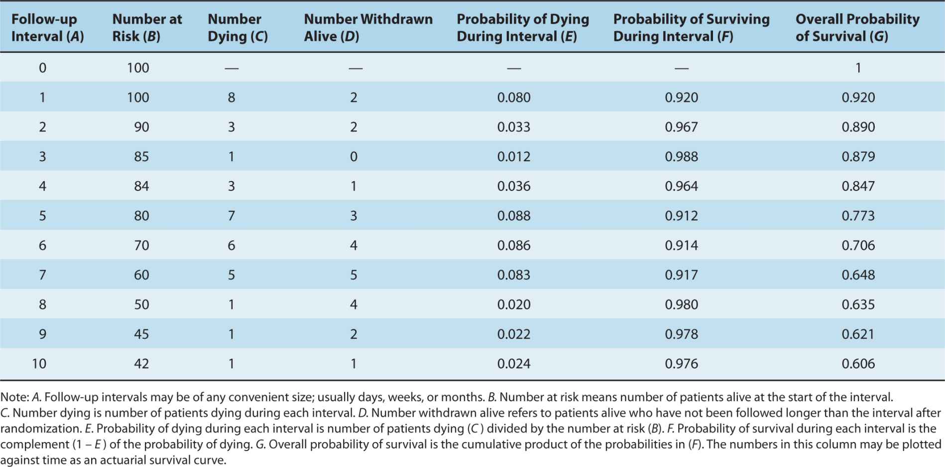
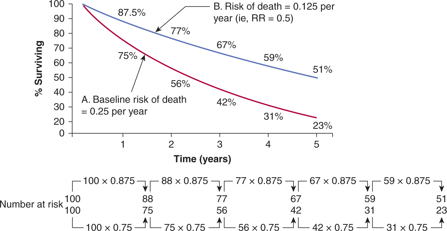
FIGURE 22–2 Hypothetical survival curves for 2 patient groups. In a 1-year interval, patients in group A have a 25% probability of dying, while those in group B have a 12.5% probability of dying (ie, relative risk [RR] = 0.5). At the end of 5 years 77% of patients in group A have died (survival rate = 23%). Note that although the hazard rate of death in group B = 0.5, by the end of 5 years, the cumulative risk of death is 49%, not 0.5 × 77% (= 38.5%).

The Kaplan-Meier method of survival analysis, also known as the product limit method, is identical to the actuarial method except that the calculations are performed at each death rather than at fixed intervals. The Kaplan-Meier survival curve is depicted graphically with the probability of survival on the y-axis and time on the x-axis: vertical drops occur at each death. The latter part of a survival curve is often the focus of most interest, as it estimates the probability of long-term survival; however, it is also the least-reliable part of the curve, because it is based on fewer observations and therefore more liable to error. The validity of all actuarial methods depends on the time of censoring being independent of the time of death; that is, those who have been followed for a short period of time or who are lost to follow-up are assumed to have similar probability of survival as those who have been followed longer. The most obvious violation of this assumption occurs if subjects are lost to follow-up because they have died or are too sick to attend clinics.

Overall survival curves do not take into account the cause of death. Cause-specific survival curves are constructed by considering only death from specified causes; patients dying from other causes are treated as censored observations at the time of their death. The advantage of cause-specific survival curves is that they focus on deaths because of the cause of interest. However, they may be influenced by uncertainty about the influence of cancer or its treatment on death because of apparently unrelated causes. Deaths from cardiovascular causes, accidents, or suicides, for example, may all occur as an indirect consequence of cancer or its treatment.

The first step in comparing survival distributions is visual inspection of the survival curves. Ideally, there will be indications of both the number of censored observations and the number of people at risk at representative time points, often indicated beneath the curve (see Fig. 22–2). Curves that cross are difficult to interpret, because this means that short-term survival is better in one arm, whereas long-term survival is better in the other. Two questions must be asked of any observed difference in survival curves: (a) whether it is clinically important and (b) whether it is likely to have arisen by chance. The first is a value judgment that will be based on factors such as absolute magnitude of the observed effect, toxicity, baseline risk, and cost of the treatment (see Sec. 22.2.10). The second is a question of statistical significance, which, in turn, depends on the size of the difference, the variability of the data, and the sample size of the trial.

The precision of an estimate of survival is conveniently described by its 95% confidence interval. Confidence intervals are closely related to p-values: a 95% confidence interval that excludes a treatment effect of zero indicates a p-value of less than 0.05. The usual interpretation of the 95% confidence interval is that there is a 95% probability that the true value of the measurement (hazard ratio, odds ratio, risk ratio) lies within the interval. The statistical significance of a difference in survival distributions is expressed by a p-value, which is the probability that a difference as large as or larger than that observed would have arisen by chance alone. Several statistical tests are available for calculating the p-value for differences in survival distributions. The log-rank test (also known as the Mantel-Cox test) and the Wilcoxon test are the most commonly used methods for analyzing statistical differences in survival curves. Both methods quantify the difference between survival curves by comparing the difference between the observed number of deaths and the number expected if the curves were equivalent. Because the Wilcoxon test gives more weight to early follow-up times when the number of patients is greater, it is less sensitive than the log-rank test to differences between survival curves that occur later in follow-up.

Survival analyses can be adjusted, in principle, for any number of prognostic variables. For example, a trial comparing the effects of 2 regimens of adjuvant chemotherapy on the survival of women with early stage breast cancer might include women with or without spread to axillary lymph nodes and with or without hormone-receptor expression. An unadjusted analysis would compare the survivals of the 2 treatment groups directly. The estimate of the treatment effect can be adjusted for any imbalances in these prognostic factors by including them in a multivariable analysis. Although simple parametric tests such as the Kaplan-Meier method can account for categorical variables, in order to assess for continuous or time-dependent variables, the more complex Cox proportional hazards model is preferred (Tibshirani, 1982; see Sec. 22.4.1 and Chap. 3, Sec. 3.3.3). In large randomized trials, such adjustments rarely affect the conclusions, because the likelihood of major imbalances is small.

Differences in the distribution of survival times for 2 treatments compared in a randomized trial may be summarized in several ways:

1. The absolute difference in the median survival or in the proportion of patients who are expected to be alive at a specified time after treatment (eg, at 5 or 10 years).

2. The hazard ratio (ratio of the probability of mortality over a specific time interval) between the 2 arms.

3. The number of patients who would need to be treated to prevent 1 death over a given period of time.

Differences in data presentation may create substantially different impressions of the clinical benefit derived from a new treatment. For example, a substantial reduction in hazard ratio may correspond to only a small improvement in absolute survival and a large number of patients who would need to be treated to save 1 life. These values depend on the expected level of survival in the control group. For example, a 25% relative improvement in overall survival has been found for use of adjuvant combination chemotherapy in younger women with breast cancer (Early Breast Cancer Trialists Collaborative Group, 2005). If this treatment effect is applied to node-positive women with a control survival at 10 years of less than 50%, it will lead to an absolute increase in survival of approximately 12%; between 8 and 9 women would need to be treated to save 1 life over that 10-year period. The same 25% reduction in hazard ratio would lead to approximately a 6% increase in absolute survival at 10 years for node-negative women where control survival at 10 years is around 75%. This corresponds to 1 life saved over 10 years for every 17 women treated. When presented with different summaries of trials, physicians may select the experimental treatment on the basis of what appears to be a substantial reduction in hazard or odds ratio, but reject treatment on the basis of a smaller increase in absolute survival or a large number of patients that need to be treated to save 1 life, even though these represent different expressions of the same effect (Chao et al, 2003). Note also that over a long time interval, the cumulative risk of death in one group cannot be determined simply by multiplying the hazard ratio by the cumulative risk of death in the baseline group. Because the number of patients at risk changes with time, the absolute gain in survival does not equal the product of this calculation (see Fig. 22–2).

22.2.6 Statistical Issues

The number of subjects required for a randomized clinical trial where the primary end point is duration of survival depends on several factors:

1. The minimum difference in survival rates that is considered clinically important: the smaller the difference, the larger the number of subjects required.

2. The number of deaths expected with the standard treatment used in the control arm: a smaller number of subjects is required when the expected survival is either very high or very low (see Table 22–4).

3. The probability of (willingness to accept) a false-positive result (alpha, or type I error): the lower the probability, the larger the number of subjects required.

4. The probability of (willingness to accept) a false-negative result (beta, or type II error): the lower the probability, the larger the number of subjects required.

TABLE 22–4 Number of patients required to detect or exclude an improvement in survival. Data assume α = 0.05; power, 1 – β = 0.90

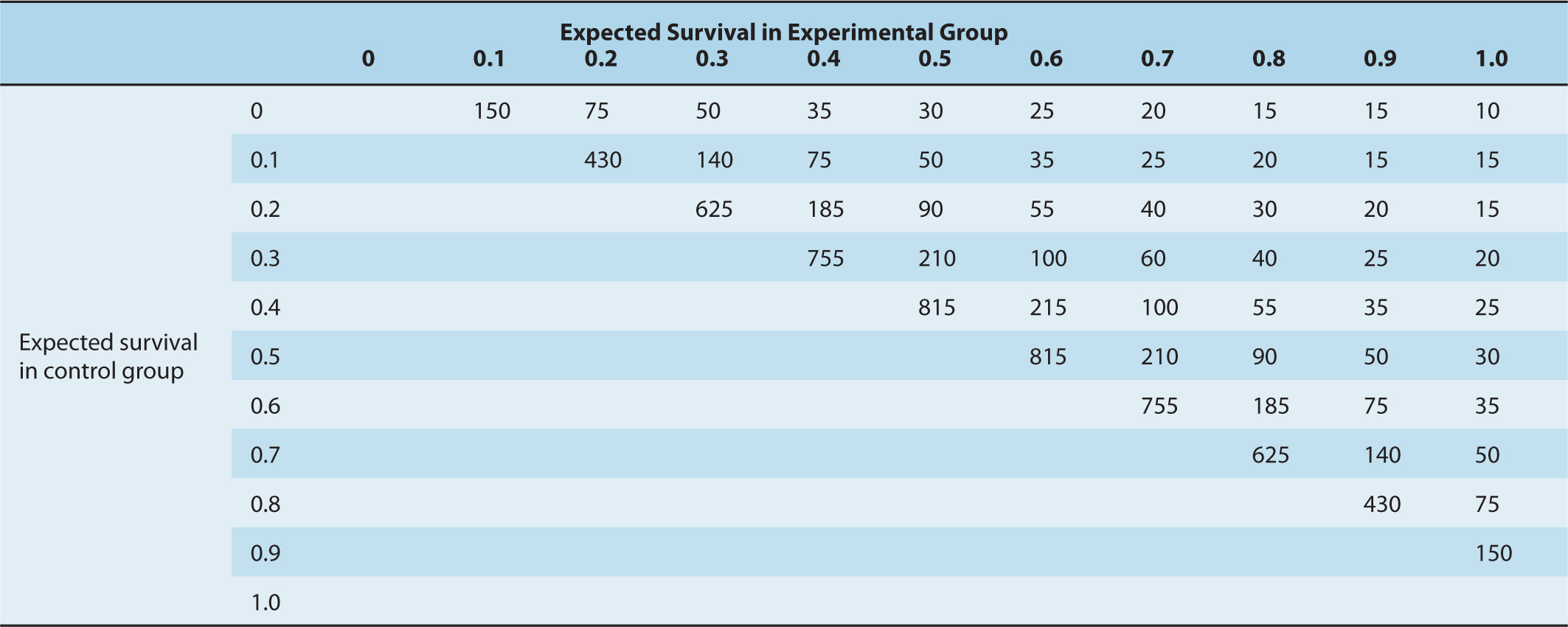
The minimum difference that is clinically important is the smallest difference that would lead to the adoption of a new treatment. This judgment will depend on the severity of the condition being treated and the feasibility, toxicity, and cost of the treatment(s). Methods are available to help quantify such judgments. For example, the practitioners who will be expected to make decisions about treatment based on the results of the trial can be asked what magnitude of improvement would be sufficient for them to change their practice by adopting the new treatment. Based on such information, the required number of patients to be entered into a trial can be estimated from tables similar to Table 22–4. The acceptable values for the error probabilities are matters of judgment. Values of 0.05 for alpha (false-positive error) and 0.1 or 0.2 for beta (false-negative error) are well-entrenched. There are good arguments for using lower (more stringent) values, although perhaps even more important is that trials should be repeated by independent investigators before their results are used to change clinical practice.

In a trial assessing survival duration, it is the number of deaths rather than the number of subjects that determines the reliability of its conclusions. For example, a trial with 1000 subjects and 200 deaths will be more reliable than a trial with 2000 subjects and 150 deaths. From a statistical point of view, this means that it is more efficient to perform trials in subjects who are at a higher risk of death than at a lower risk of death. It also explains the value of prolonged follow-up—longer follow-up means more deaths, which produce more reliable conclusions.

22.2.6.1 Power The power of a trial refers to its ability to detect a difference between treatments when in fact they do differ. The power of a trial is the complement of beta, the type II error (power = 1 – beta). Table 22–4 shows the relationship between the expected difference between treatments and the number of patients required. A randomized clinical trial that seeks to detect an absolute improvement in survival of 20%, compared with a control group receiving standard treatment whose expected survival is 40%, will require approximately 108 patients in each arm at α = 0.05 and a power of 0.9. This means that a clinical trial of this size has a 90% chance of detecting an improvement in survival of this magnitude. Detection of a smaller difference between treatments—for example, a 10% absolute increase in survival—would require approximately 410 patients in each arm. A substantial proportion of published clinical trials are too small to detect clinically important differences reliably. This may lead to important deficiencies in the translation of clinical research into practice. If an underpowered study finds “no statistically significant difference” associated with the use of a given treatment, the results may mask a clinically important therapeutic gain that the trial was unable to detect. If there are insufficient patients to have an 80% to 90% chance of detecting a worthwhile difference in survival, then a trial should probably not be undertaken. In contrast some trials, especially those sponsored by pharmaceutical companies, have become so large that they can detect very small differences in survival, which are statistically significant but may not be clinically meaningful. For example, in the National Cancer Institute of Canada PA3 trial, investigators reported a statistically significant improvement in overall survival. However, in absolute terms this amounted to an improvement in median survival of around 11 days and came at the cost of increased toxicity and treatment-related death (Moore et al, 2007).

22.2.7 Metaanalysis

Metaanalysis is a method by which data from individual randomized clinical trials that assess similar treatments (eg, adjuvant chemotherapy for breast cancer versus no chemotherapy) are combined to give an overall estimate of treatment effect. Metaanalysis can be useful because (a) the results of individual trials are subject to random error and may give misleading results, and (b) a small effect of a treatment (eg, approximately 5% improvement in absolute survival for node-negative breast cancer from use of adjuvant chemotherapy) may be difficult to detect in individual trials. Detection of such a small difference will require several thousand patients to be randomized, yet it may be sufficiently meaningful to recommend adoption of the new treatment as standard.

Metaanalysis requires the extraction and combination of data from trials addressing the question of interest. The preferred method involves collection of data on individual patients (date of randomization, date of death, or date last seen if alive) that were entered in individual trials, although literature-based approaches are also recognized. The trials will, in general, compare related strategies of treatment to standard management (eg, radiotherapy with or without chemotherapy for stage III non–small cell lung cancer) but may not be identical (eg, different types of chemotherapy might be used).

Metaanalysis is typically a 2-stage process. First, summary statistics (such as risk or hazard ratios) are calculated for individual studies. Then a summary (pooled) effect estimate is calculated as a weighted average of the effects of the intervention in the individual studies. There are 2 models for weighting studies in the pooled estimate. If each study is assumed to estimate the same relative outcome such that there is no interstudy heterogeneity, then any error is derived from measurement error within individual studies, and studies are weighted by their sample size. In studies not all estimating the same outcome, it is assumed that interstudy variability is more significant than intrastudy variability and a random-effects metaanalysis is carried out, which weights most studies equally regardless of their size. All methods of metaanalysis should incorporate a test of heterogeneity—an assessment of whether the variation among the results of the separate studies is compatible with random variation, or whether it is large enough to indicate inconsistency in the effects of the intervention across studies (interaction).

Data are presented typically in forest plots as in Figure 22–3, which illustrates the comparison of a strategy (in this example, ovarian ablation as adjuvant therapy for breast cancer) used alone versus no such treatment (upper part of figure) and a related comparison where patients in both arms also receive chemotherapy (lower part of figure). Here, each trial included in the metaanalysis is represented by a symbol, proportional in area to the number of patients on the trial, and by a horizontal line representing its confidence interval. A vertical line represents the null effect, and a diamond beneath the individual trials represents the overall treatment effect and confidence interval. If this diamond symbol does not intersect the vertical line representing the null effect, a significant result is declared.

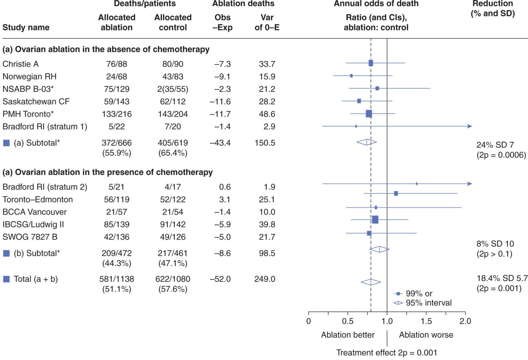
FIGURE 22–3 Presentation of results of a metaanalysis in a forest plot. Each trial is represented by a square symbol, whose area is proportional to the number of patients entered, and by a horizontal line. These represent the mean and 95% confidence interval for the ratio of annual odds of death in the experimental and standard arms. A vertical line drawn through odds ratio 1.0 represents no effect. The trials are separated into those asking a simple question (in this example, ovarian ablation versus no adjuvant treatment for early breast cancer) and a related but more complex question (ovarian ablation plus chemotherapy versus chemotherapy alone). Diamonds represent overall mean odds ratios and their 95% confidence intervals for the 2 subsets of trials and for overall effect. The vertical dashed line represents mean reduction in annual odds of death for all trials. (Adapted from Early Breast Cancer Trialists Collaborative Group, 1996.)

The potential for bias and methodological quality can be assessed in a metaanalysis. A funnel plot is a simple scatter plot in which a measure of each study’s size or precision is plotted against a measure of the effect of the intervention. Symmetrical funnel plots suggest, but do not confirm absence of bias and high methodological quality. Sources of asymmetry in funnel plots include selection biases (such as publication bias: that is, the tendency for preferential and earlier publication of positive studies, and selective reporting of outcomes), poor methodological quality leading to spuriously inflated effects in smaller studies, inadequate analysis, or fraud.

Metaanalysis is an expensive and time-consuming procedure. Important considerations are as follows:

1. Attempts should be made to include the latest results of all trials; unpublished trials should be included to avoid publication bias.

2. Because of publication bias and other reasons, metaanalyses obtained from reviews of the literature tend to overestimate the effect of experimental treatment as compared with a metaanalysis based on data for individual patients obtained from the investigators (Stewart and Parmar, 1993).

3. Because metaanalysis may combine trials with related but different treatments (eg, less-effective and more-effective chemotherapy), the results may underestimate the effects of treatment that could be obtained under optimal conditions.

There is extensive debate in the literature about the merits and problems of metaanalyses and their advantages and disadvantages as compared with a single, large, well-designed trial (Parmar et al, 1996; Buyse et al, 2000; Noble, 2006). A well-performed metaanalysis uses all the available data, recognizes that false-negative and false-positive trials are likely to be common, and may limit the inappropriate influence of individual trials on practice.

22.2.8 Patient-Reported Outcomes

Physician-evaluated performance status and patient reported outcomes such as quality of life are correlated, but are far from identical, and both can provide independent prognostic information in clinical trials (see Sec. 22.4.3). Patient-reported outcomes include symptom scales (eg, for pain or fatigue) and measures of quality of life. Physicians and other health professionals are quite poor in assessing the level of symptoms of their patients, and simple methods for grading symptoms by patients, such as the Functional Assessment of Cancer Therapy (FACT) Scale or the Edmonton Symptom Assessment Scale (Cella et al, 1993; Nekolaichuk et al, 1999) can give valuable information about palliative (or toxic) effects on patients with cancer who are participating in clinical trials. Quality of life is an abstract, multidimensional concept reflecting physical, psychological, spiritual, and social aspects of life that includes but is not limited to the concept of health. It reflects an individual’s perception of and response to his or her unique circumstances. This definition gives primacy to the individual’s views and self-assessment is essential. Instruments (questionnaires) addressing differing aspects of quality of life from a variety of perspectives are now available. Questionnaires range from generic instruments designed for people with a variety of conditions or diseases to instruments designed for patients with a specific type and stage of cancer. The FACT–General (FACT-G), developed for people receiving cancer treatments (Cella et al, 1993); and the European Organization for Research and Treatment of Cancer Core Quality of Life Questionnaire (EORTC QLQ-C30), developed for people with cancer participating in international clinical trials (Aaronson et al, 1993) are used most often to evaluate people with cancer. Both combine a core questionnaire relevant to most patients with cancer, as well as an increasing number of subscales that allow subjects to evaluate additional disease or symptom-specific items.

The validity of an instrument refers to the extent to which it measures what it is supposed to measure. The validity of a quality-of-life instrument is always open to question, as there is no objective, external gold standard for comparison. Instead, a variety of indirect methods are used to gauge the validity of quality-of-life instruments (Aaronson et al, 1993). Examples include convergent validity, the degree of correlation between instruments or scales purporting to measure similar attributes; and discriminant validity or the degree to which an instrument can detect differences between different aspects of quality of life. Face validity and content validity refer to the extent to which an instrument addresses the issues that are important. Responsiveness refers to the detection of changes in quality of life with time, such as those caused by effective treatment, while predictive validity refers to the prognostic information of a quality-of-life scale in predicting an outcome such as duration of survival. Validated quality-of-life scales are often strong predictors of survival (see Sec. 22.4.3).

Validity is conditional—it cannot be judged without specifying for what and for whom it is to be used. Good validity of a questionnaire in symptomatic men with advanced hormone-resistant prostate cancer does not guarantee good validity in men with earlier-stage prostate cancer, for whom pain might be less important and sexual function more important. Even within the same population of subjects, differences between interventions, such as toxicity profiles, might influence validity. For example, nausea and vomiting might be important in a trial of cisplatin-based chemotherapy, whereas sexual function might be more important in a trial of hormonal therapy. The context in which an instrument is to be used and the context(s) in which its validity was assessed must be reexamined for each application. Furthermore, it is important that an a priori hypothesis for palliative end points is defined and preferable that the proportion of patients with palliative response is reported (Joly et al, 2007).

There are methodological challenges to using patient-reported outcomes such as quality-of-life data. There is little evidence to inform the optimal timing for assessment and the intervals at which assessments should be repeated. Attrition because of incomplete data collection remains a challenge and can confound quality-of-life analysis (patients with poor quality of life are less likely to complete questionnaires). Patient perceptions of their quality of life can change over time (eg, “good quality of life” may be quite different for a patient who has lived with cancer for several years as compared to someone without the disease; this is known as response-shift). Psychological defenses also tend to conserve perception of good quality of life even in the presence of worsening symptoms (Sprangers, 1996).

22.2.9 Health Outcomes Research

Outcomes research seeks to understand the end results of various factors on patients and populations. It can be used to assess prognostic factors, such as the effect of socioeconomic status on cancer survival (Booth et al, 2010), studies that compare different approaches to the management of specific medical conditions, studies that examine patients’ and clinicians’ decision making, studies describing geographic variations in clinical practice, and studies to develop or test practice guidelines. Outcomes research usually addresses the interrelated issues of cost and quality of health care, and public and private sector interest. The availability of computer methods to link large data bases (eg, cancer incidence and mortality data from cancer registries and treatment data from hospital records) has facilitated the ability of health outcomes research to address important clinical questions.

Various methodological designs are utilized in outcomes research. These include cohort studies, case-control studies, and studies of the uptake and outcome of new evidence-based treatment for management (also called phase 4 studies). These studies can be undertaken prospectively or retrospectively. End points in outcomes research are usually clinical, economic, or patient-centered. Clinical outcomes include mortality or medical events as a result of an intervention. Economic outcomes include direct health costs (eg, costs of medical care, see Sec. 22.2.10), direct nonhealth costs (eg, cost of care providers), indirect costs (eg, productivity costs) and intangible costs (eg, pain and suffering). Patient-centered outcomes include quality of life and patient satisfaction. In most studies, the focus is on clinical outcomes. A major difference between outcomes research and randomized trials is that outcomes research lacks the controls and highly structured and artificial environment. An example of the utility of outcomes research comes from the Prostate Cancer Outcomes Study. In this project, the Surveillance, Epidemiology, and End Results (SEER) database of the United States National Cancer Institute was used to assess the outcomes of approximately 3500 men who had been diagnosed with primary invasive prostate cancer. Unlike many randomized trials, this study included a substantial number of men of different ethnic origins and socioeconomic groups, who had been treated in a variety of settings. This methodology enabled investigators to assess racial differences in stage at diagnosis and in treatment to help explain the significantly higher mortality rates from prostate cancer among black men in the United States (Hoffman et al, 2001).

The gold standard for assessing a medical intervention remains the randomized trial. However, randomized trials are not feasible in all settings and such trials tend to be conducted in highly selected populations and their results are not always applicable to the general population. Outcomes research aims to bridge the transition from research that is designed to assess the efficacy and safety of medical interventions to research that is undertaken under real-world conditions to evaluate their effectiveness in normal clinical practice. Health outcomes research has a number of advantages over traditional controlled trials, such as a lack of selection bias and the ability to generalize results to the real world. These advantages make outcomes research more helpful in assessing societal benefit from medical intervention than controlled trials. Disadvantages to outcomes research include lack of randomized comparisons and the likelihood that causality may be attributed to several interventions, not only the one of interest. An example of this is the exploration of screening mammography for breast cancer. Outcomes data show improved outcomes after the introduction of screening in many populations. Unfortunately, it remains unclear whether the improved outcomes can be associated with mammography alone or a combination of mammography, improvements in treatment and patient awareness and the establishment of multidisciplinary teams (Welch, 2010).

22.2.10 Cost-Effectiveness

Pharmacoeconomic evaluations play an integral role in the funding decisions for cancer drugs. The basic premise of the evaluation of cost-effectiveness is to compare the costs and consequences of alternative interventions, and to determine which treatment offers best value for limited resources. There are several methods available to evaluate economic efficiency, including cost minimization, cost benefit, and cost effectiveness analysis (Canadian Agency for Drugs and Technology in Health, 2006; Shih and Halpern, 2008). With respect to anticancer drugs, cost utility analysis (a type of cost-effectiveness analysis) is the preferred method because it considers differences in cost, survival, and quality of life between 2 competing interventions. In its most common form, a new strategy is compared to a reference standard to calculate the incremental cost-effectiveness ratio (ICER):

In Equation 22.1, the ICER may be expressed as the increased cost per life-year gained, which can be estimated from differences in survival when the new treatment is compared with the standard treatment in a randomized controlled led trial. The increase in survival can be adjusted for differences in quality of survival by multiplying the median survival with each treatment by the “utility” of the survival state, where “utility” is a factor between zero and 1 that is a measure of the relative quality of life of patients following each treatment (as compared to perfect health) (Shih and Halpern, 2008). The ICER is then expressed as the increased cost to gain 1 quality-adjusted life-year (QALY); in practice, utility is often difficult to estimate, and in the absence of major differences in toxicity between new and standard treatment, the simpler increase in cost-per-life-year gained is often used.

If the ICER falls below a predefined threshold, the new treatment is considered cost-effective, otherwise it is considered cost-ineffective. A major challenge in the use of pharmacoeconomic modeling for estimating drug cost is in establishing the threshold for value. For example, the National Institute for Clinical Excellence in the United Kingdom has established a threshold ICER of £30,000 (~US$50,000) per QALY gained (Devlin and Parkin, 2004). In many other jurisdictions, a similar US$50,000 threshold has been used (Laupacis et al, 1992). There remains no consensus as to what threshold is appropriate, but by convention, cutoffs of $50,000 to $100,000 per QALY are often used for public funding of new treatments in developed countries; much lower costs per QALY can be supported in the developing world (Sullivan et al, 2011).

In principle, the added costs per QALY gained can be used by public health systems to make choices between funding quite different health interventions. For example, a health jurisdiction might compare the cost effectiveness ratio from extending the use of coronary artery bypass surgery to that from introduction of a new anticancer drug, and select that which provides the lower cost for a given increase in QALYs or life-years.

22.3 DIAGNOSIS AND SCREENING

22.3.1 Diagnostic Tests

Diagnostic tests are used to screen for cancer in people who are symptom free, establish the existence or extent of disease in those suspected of having cancer, and follow changes in the extent and severity of the disease during therapy or follow-up. Diagnostic tests are used to distinguish between people with a particular cancer and those without it. Test results may be expressed quantitatively on a continuous scale or qualitatively on a categorical scale. The results of serum tumor marker tests, such as PSA, are usually expressed quantitatively as a concentration, whereas the results of imaging tests, such as a computed tomography (CT) scan, are usually expressed qualitatively as normal or abnormal. To assess how well a diagnostic test discriminates between those with and without disease, it is necessary to have an independent means of classifying those with and without disease—a “gold standard.” This might be the findings of surgery, the results of a biopsy, or the clinical outcome of patients after prolonged follow-up. If direct confirmation of the presence of disease is not possible, the results of a range of different diagnostic tests may be the best standard available.

Simultaneously classifying the subjects into diseased (D+) and nondiseased (D–) according to the gold-standard test and positive (T+) or negative (T–) according to the diagnostic test being assessed defines 4 subpopulations (Fig. 22–4). These are true-positives (TPs: people with the disease in whom the test is positive), true-negatives (TNs: people without the disease in whom the test is negative), false-positives (FPs: people without the disease in whom the test is positive), and false-negatives (FNs: people with the disease in whom the test is negative).

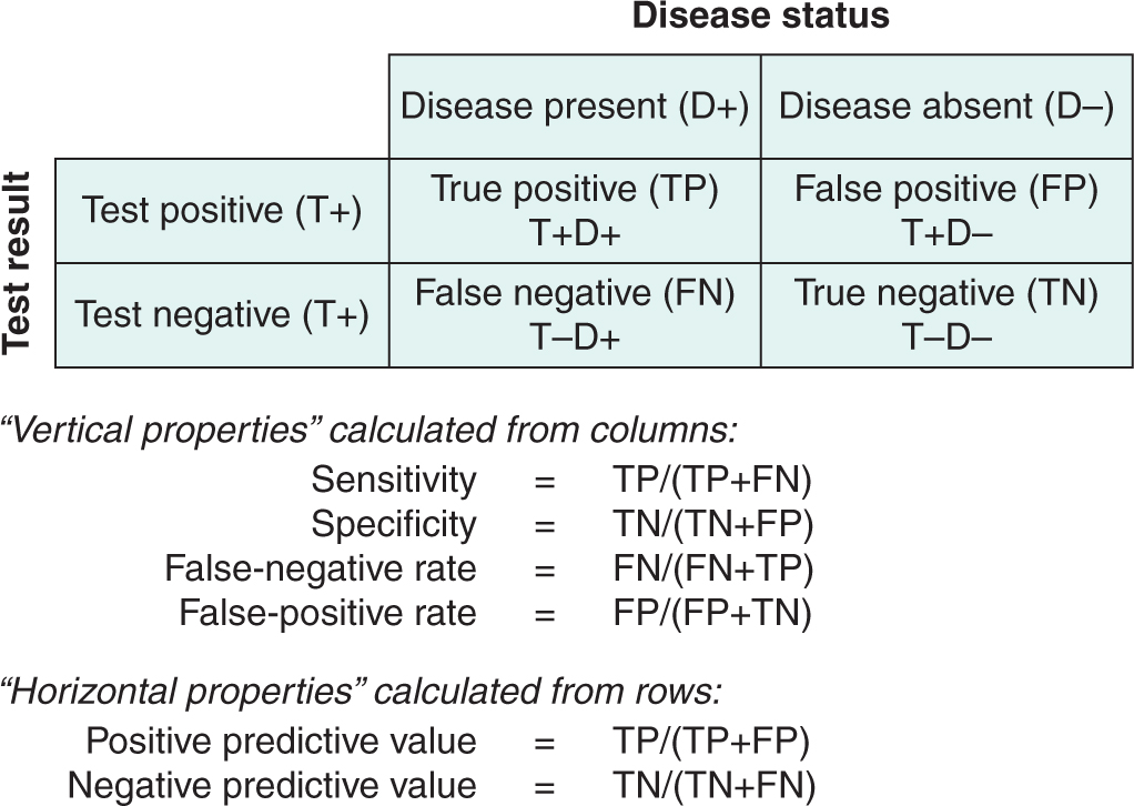
FIGURE 22–4 Selection of a cutoff point for a diagnostic test defines 4 subpopulations as shown. Predictive values (but not sensitivity and specificity) depend on the prevalence of disease in the population tested.

Test performance can be described by indices calculated from the 2 × 2 table shown in Figure 22–4. “Vertical” indices are calculated from the columns of the table and describe the frequency with which the test is positive or negative in people whose disease status is known. These indices include sensitivity (the proportion of people with disease who test positive) and specificity (the proportion of people without disease who test negative). These indices are characteristic of the particular test and do not depend on the prevalence of disease in the population being tested. The sensitivity and specificity of a test can be applied directly to populations with differing prevalence of disease.

“Horizontal” indices are calculated from the rows of the table and describe the frequency of disease in individuals whose test status is known. These indices indicate the predictive value of a test—for example, the probability that a person with a positive test has the disease (positive predictive value) or the probability that a person with a negative test does not have the disease (negative predictive value). These indices depend on characteristics of both the test (sensitivity and specificity) and the population being tested (prevalence of disease in the study population). The predictive value of a test cannot be applied directly to populations with differing prevalence of disease.

Figure 22–5 illustrates the influence of disease prevalence on the performance of a hypothetical test assessed in populations with high, intermediate, and low prevalence of disease. Sensitivity and specificity are constant, as they are independent of prevalence. As the prevalence of disease declines, the positive predictive value of the test declines. This occurs because, although the proportions of TP results among diseased subjects and FP results among nondiseased subjects remain the same, the absolute numbers of TP and FP results differ. In Figure 22–5, in the high-prevalence population, the absolute number of false positives (10) is small in comparison with the absolute number of true positives (80): a positive result is 8 times more likely to come from a subject with disease than a subject without disease, and the positive predictive value of the test is relatively high. In the low-prevalence population, the absolute number of false positives (1000) is large in comparison with the absolute number of true positives (80): a positive result is 12.5 times more likely to come from a subject without disease, and the positive predictive value is relatively low. For this reason, diagnostic tests that may be useful in patients where there is already suspicion of disease (high-prevalence situation) may not be of value as screening tests in a less selected population (low-prevalence situation; see Sec. 22.3.3).

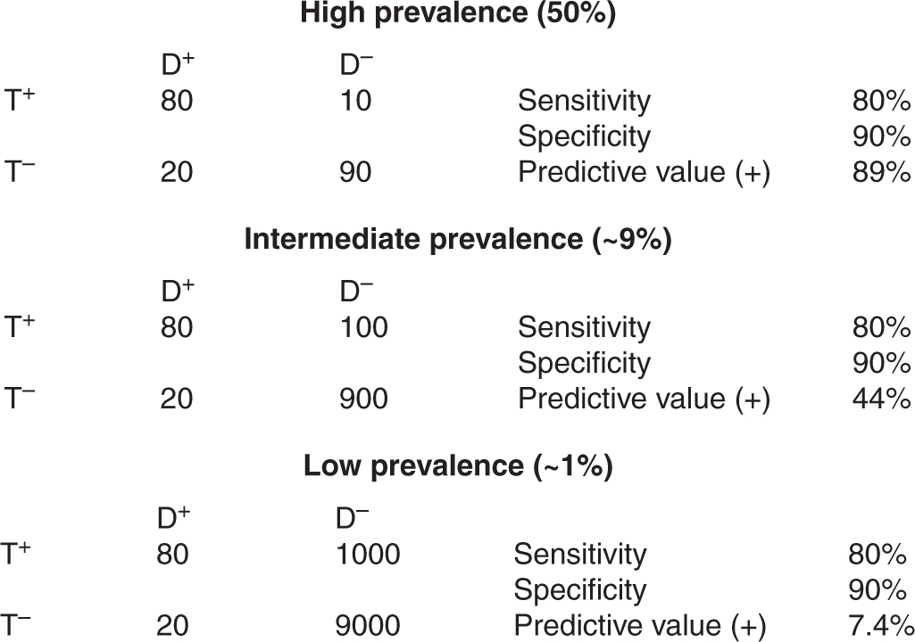
FIGURE 22–5 Test properties and disease prevalence. Examples of application of a diagnostic test to populations in which disease has high, intermediate, or low prevalence. The predictive value of the test decreases when there is a low prevalence of disease.

If a quantitative test is to be used to distinguish subjects with or without cancer, then a cutoff point must be selected that distinguishes positive results from negative results. Quantitative test results are often reported with a normal or reference range. This is the range of values obtained from some arbitrary proportion, usually 95%, of apparently healthy individuals; the corollary is that 5% of apparently healthy people will have values outside this range. Diagnostic test results are rarely conclusive about the presence or absence of diseases such as cancer; more often, they just raise or lower the likelihood that it is present.

Figure 22–6 shows the effects of choosing different cutoff points for a diagnostic test. A cutoff point at level A provides some separation of subjects with and without cancer, but because of overlap, there is always some misclassification. If the cutoff point is increased to level C, fewer subjects without cancer are wrongly classified (ie, the specificity increases) but more people with cancer fall below the cutoff and will be incorrectly classified (ie, the sensitivity decreases). A lower cutoff point at level B has the opposite effect: More subjects with cancer are correctly classified (sensitivity increases), but at the cost of incorrectly classifying larger numbers of people without cancer (specificity decreases). This trade-off between sensitivity and specificity is a feature of all diagnostic tests.

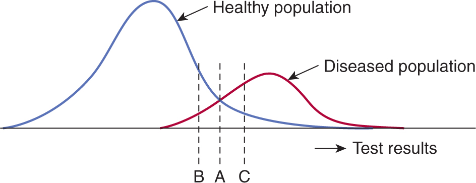
FIGURE 22–6 Interpretation of a diagnostic test (eg, PSA for prostate cancer) requires the selection of a cutoff point that separates negative from positive results. The position of the cutoff point (which might be set at A, B, or C) influences the proportion of patients who are incorrectly classified as being healthy or having disease.

The 2 × 2 table and the indices derived from it (see Fig. 22–4) provide a simple and convenient method for describing test performance at a single cutoff point, but they give no indication of the effect of using different cutoff points. A receiver operating characteristic (ROC) curve provides a method for summarizing the effects of different cutoff points on sensitivity, specificity, and test performance. Figure 22–7 shows examples of ROC curves. The ROC curve plots the true-positive rate (TPR; which equals sensitivity) against the false-positive rate (FPR; which equals 1 – specificity) for different cutoff values. The “best” cutoff point is the one that offers the best compromise between TPR and FPR. This is represented by the point on the ROC curve closest to the upper left-hand corner. Statistically, ROC curves represent the balance between sensitivity and specificity with the area under the ROC curve (AUC; also known as the C-statistic) showing a model’s discriminatory accuracy. An AUC of 0.5 is no better than a flip of a coin, whereas an AUC of 1.0 represents a perfect test. Realistically, an AUC of 0.7 or 0.8 is consistent with good discriminatory accuracy.

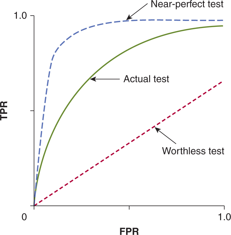
FIGURE 22–7 Curves showing ROCs in which the true-positive rate (TPR) is plotted against the false-positive rate (FPR) of a diagnostic test as the cutoff point is varied. The performance of the test is indicated by the shape of the curve, as shown.

22.3.2 Sources of Bias in Diagnostic Tests

The performance of a diagnostic test is usually evaluated in a research study to estimate its usefulness in clinical practice. Differences between the conditions under which a test is evaluated, and the conditions under which it will be used, may produce misleading results. Important factors relating both to the people being tested and the methods being used are summarized in Table 22–5 (see also Jaeschke et al, 1994, and Scales et al, 2008). If a test is to be used to identify patients with colon cancer, then the study sample should include people with both localized and advanced disease (a wide clinical spectrum). The sample should also include people with other clinical conditions that might be mistaken for colon cancer (eg, diverticular disease) in order to evaluate the ability of the test to distinguish between these conditions, or to detect colon cancer in its presence (comorbidity). If there are different histological types of a cancer, then the test should be evaluated in a sample of patients that have these different histological types.

TABLE 22–5 Factors that may distort the estimated performance of a diagnostic test.

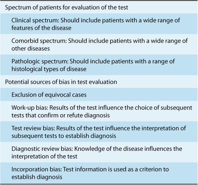
The evaluation of diagnostic test performance requires subjects to be classified by both disease status (diseased or nondiseased) and test status (positive or negative). For the evaluation to be valid, the 2 acts of classification must be independent. If either the classification of disease status is influenced by the test result or the interpretation of the test result is influenced by disease status, then there will be an inappropriate and optimistic estimate of test performance (see below and Table 22–5).

Work-up bias arises if the results of the diagnostic test under evaluation influence the choice of other tests used to determine the subject’s disease status. For example, suppose that the performance of a positron emission tomographic (PET) scan is to be evaluated as an indicator of spread of hitherto regional lung cancer by comparing it with the results of mediastinal lymph node biopsy. Work-up bias will occur if only patients with abnormal PET scans are selected for mediastinoscopy, because regional spread in patients with normal PET scans will remain undetected. This leads to an exaggerated estimate of the predictive value of PET scanning.

Test-review bias occurs when the subjective interpretation of one test is influenced by knowledge of the result of another test. For example, a radiologist’s interpretation of a PET scan might be influenced by knowledge of the results of a patient’s CT scan. Using the CT scan to help interpret the results of an ambiguous PET scan may lead to a systematic overestimation of the ability of PET scan to identify active tumor. The most obvious violation of independence of the test and the method used to establish diagnosis arises when the test being evaluated is itself incorporated into the classification of disease status.

Diagnostic-review bias occurs when the reference test results are not definitive and the study test results affect or influence how the final diagnosis is established (Begg and McNeil, 1988).

22.3.3 Tests for Screening of Disease

Diagnostic tests are often used to screen an asymptomatic population to detect precancerous lesions or early cancers that are more amenable to treatment than cancers detected without screening. There are factors that influence the value of a screening program other than the sensitivity and specificity of the screening test. First, the cancer must pass through a pre-clinical phase that can be detected by the screening test. Slowly growing tumors are more likely to meet this criterion. Second, treatment must be more effective for screen-detected patients than for those treated after symptoms develop: If the outcome of treatment is uniformly good or bad regardless of the time of detection, then screening will be of no benefit. Third, the prevalence of disease in the population must be sufficient to warrant the cost of a screening program. Finally, the screening test must be acceptable to the target population: painful and inconvenient tests are unlikely to be accepted as screening tools by asymptomatic individuals.

The primary goal of a screening program is to reduce disease-specific mortality, that is, the proportion of people in a population who die of a given cancer in a specified time. For disease-specific mortality, the denominator is the whole population; it is therefore independent of factors that influence the time of diagnosis of disease. Other end points often reported in screening studies include stage of diagnosis and case fatality rate (the proportion of patients with the disease who die in a specified period). However, these intermediate end points are affected by several types of bias, particularly length-time bias and lead-time bias.

Length-time bias is illustrated in Figure 22–8. The horizontal lines in the figure represent the length of time from inception of disease to the time it produces clinical signs or symptoms and would be diagnosed in the absence of screening. Long lines indicate slowly progressing disease and short lines indicate rapidly progressing disease. A single examination, such as screening for breast cancer with mammography (represented in the figure by the dashed vertical line), will intersect (detect) a larger number of long lines (people with indolent disease) than short lines (people with aggressive disease). Thus, a screening examination will selectively identify those people with slowly progressing disease.

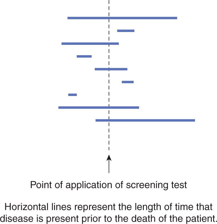
FIGURE 22–8 Illustration of length-time bias in a screening test. The test is more likely to detect disease that is present for a long time (ie, slowly growing disease). Horizontal lines represent the length of time that disease is present prior to clinical diagnosis.

Lead-time bias is illustrated in Figure 22–9. The purpose of many diagnostic tests, and of all tests that are used to screen healthy people, is to allow clinicians to identify disease at an earlier stage in its clinical course than would be possible without the test. Four critical time points in the clinical course of the disease are indicated in Figure 22–9: the time of disease inception (0), the time at which the disease becomes incurable (1), the time of diagnosis (2), and the time of death (3). Many patients with common cancers are incurable by the time their disease is diagnosed, and the aim of a screening test is to advance the time of diagnosis to a point where the disease is curable. Even if the cancer is incurable despite the earlier time of diagnosis, survival will appear to be prolonged by early detection because of the additional time (the lead-time) that the disease is known to be present (Fig. 22–9). In screening for breast cancer with mammography, the lead-time is estimated to be approximately 2 years. Advancing the date of diagnosis may be beneficial if it increases the chance of cure. However, if it does not increase the chance of cure, then advancing the date of diagnosis may be detrimental, because patients spend a longer time with the knowledge that they have incurable disease.

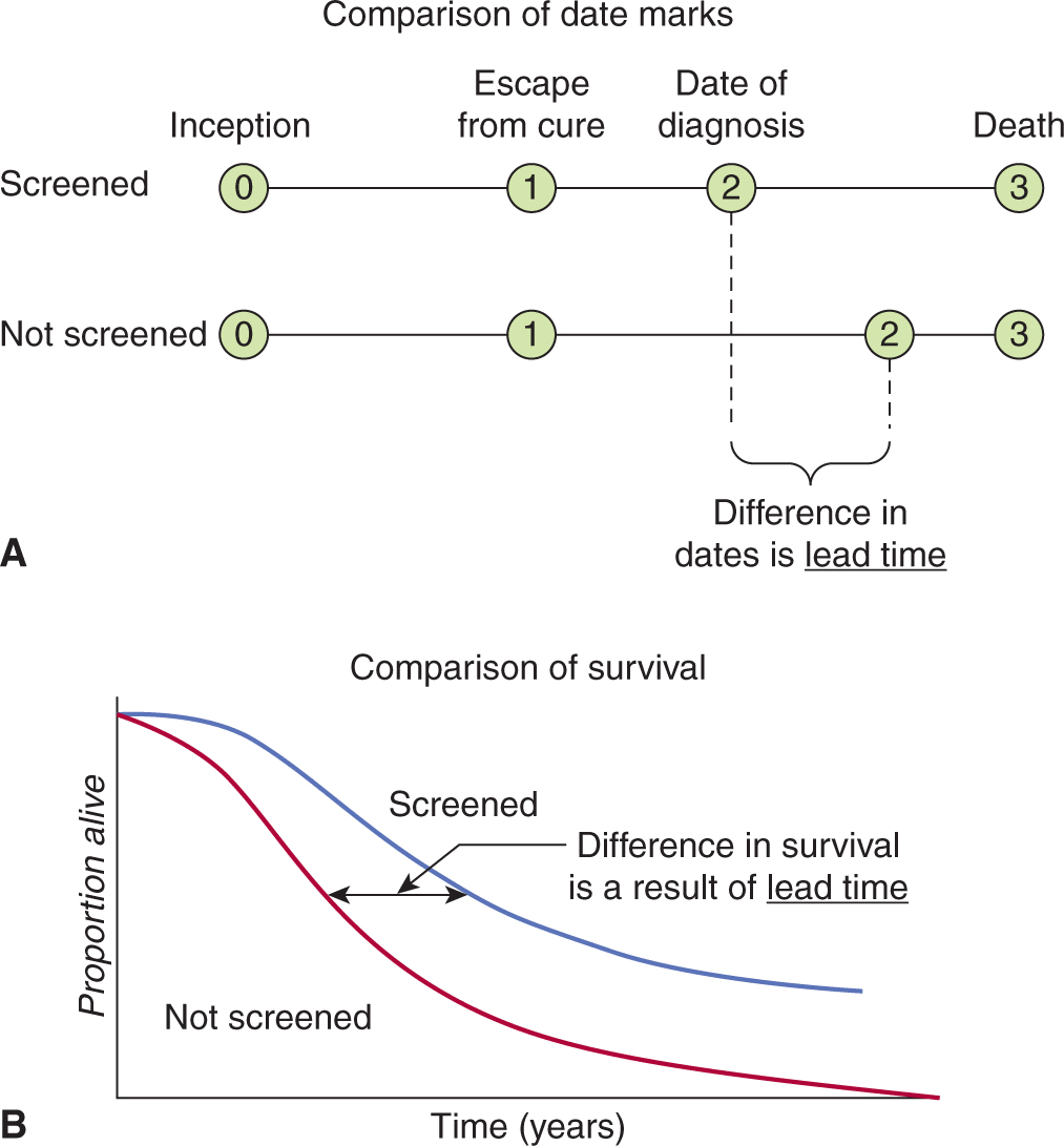
FIGURE 22–9 Illustration of lead-time bias. A) Application of a test may lead to earlier diagnosis without changing the course of disease. B) There is an improvement in survival when measured from time of diagnosis.

The strongest study design for evaluating the impact of a diagnostic or screening test involves the randomization of people to have the test or to be followed in the usual way without having the test. The most important outcome measures that are assessed in such a trial include overall survival, disease-specific survival, and quality of life. Both randomized trials and those using health outcomes methods have demonstrated reductions in mortality rates as a result of breast cancer associated with mammographic screening in postmenopausal women (Kalager et al, 2010) and with fecal occult blood testing for colorectal carcinoma (Towler et al, 1998). However, an overview of the quality of trials of screening mammography has questioned whether there is a true reduction in mortality (Olsen and Gotzsche, 2001). Also, there has been a decrease in disease-specific mortality, but an increase in death rate from all causes in some trials (Black et al, 2002). Some screening procedures might be harmful in that they lead to investigations with some associated morbidity and mortality. Randomized trials have demonstrated a small benefit associated with screening people at high risk for lung cancer using spiral CT scans (National Lung Screening Trial, 2010), while trials evaluating the value of PSA screening for prostate cancer have either shown no benefit or a small decrease in disease-specific mortality (Andriole et al, 2009; Schröder et al, 2009).

22.3.4 Diagnostic Tests During Follow-up of Treated Tumors

Among patients who have had a complete response to treatment, most follow-up tests can be viewed as a form of screening for local or metastatic recurrence. Consequently, many of the requirements for an effective screening test described above also apply to follow-up tests. Because most recurrent cancers are not curable (particularly metastatic recurrences), it is uncommon that early intervention to treat asymptomatic recurrence will produce a true improvement in mortality due to disease. Studies of follow-up tests that report improvement in case-fatality rates usually suffer from lead-time bias. As with screening studies, randomized trials provide the best methodology to compare the utility of alternative approaches to follow-up. Four randomized, controlled clinical trials involving 3055 women with breast cancer, found no difference in overall survival or DFS between patients observed with intensive radiological and laboratory testing and those observed with clinical visits and mammography (Rojas et al, 2005). These findings demonstrate that for follow-up tests to improve survival, they must detect recurrences for which curative treatment is available; unfortunately, for most common tumors in adults such treatment is rarely available.

22.3.5 Bayes Theorem and Likelihood Ratios

The results of diagnostic tests are rarely conclusive about the presence or absence of disease and prognostic tests are rarely definitive about the course of disease. The utility of these tests is that they raise or lower the probability of observing a particular disease or prognosis (Jaeschke et al, 1994). This concept is embodied in the Bayes theorem. This theorem allows an initial estimate of a probability to be adjusted to take account of new information from a diagnostic or prognostic test, thus producing a revised estimate of the probability. The initial estimate is referred to as the prior or pretest probability; the revised estimate is the posterior or posttest probability.

For example, the pretest probability of breast cancer in a 45-year-old American woman presenting for screening mammography is approximately 3 in 1000 (the prevalence of disease in women of this age). If her mammogram is reported as “suspicious for malignancy,” then her posttest probability of having breast cancer rises to approximately 300 in 1000, whereas if the mammogram is reported as “normal,” then her posttest probability of having breast cancer falls to approximately 0.4 in 1000 (Kerlikowske et al, 1996).

Bayes theorem describes the mathematical relationship between the new posttest probability, the former prior probability (ie, the prevalence of disease in the tested population), and the additional information provided by a test (or clinical trial). This relationship can be expressed with 2 formulas that look different but are logically equivalent. For a diagnostic test with the characteristics defined in Figure 22–4, the probability form of Bayes’ theorem can be expressed as

The alternative form of the Bayes theorem is expressed in terms of a likelihood ratio and is much easier to use. The likelihood ratio is a useful concept that for any test result represents the ratio of the probability that disease is present to the probability that it is absent. For a positive diagnostic test, the likelihood ratio is the likelihood that the positive test represents a true positive rather than a false positive:

For a negative diagnostic test, the likelihood ratio is the likelihood that the negative result represents a false negative rather than a true negative (ie, false negative rate/true negative rate). A good diagnostic test has a high likelihood ratio for a positive test (ideally >10) and a low likelihood ratio for a negative test (ideally <0.1).

22.4 PROGNOSIS

A prognosis is a forecast of expected course and outcome for a patient with a particular stage of disease. It may apply to the unique circumstances of an individual or to the general circumstances of a group of individuals. People with apparently similar types and stages of cancer live for different lengths of time, have different patterns of progression, and respond differently to the same treatments. Variables associated with the outcome of a disease that can account for some of this heterogeneity are known as prognostic factors, and they may relate to the tumor, the host, or the environment. An increasing number of tumor-related factors, including various gene signatures (see Sec. 22.5; Chap. 2, Sec. 2.7.2), have been found to convey prognostic information.

Differences in prognostic characteristics often account for larger differences in outcome than do differences in treatment. For example, in women with primary breast cancer, differences in survival according to lymph node status are much greater than differences in survival according to treatment. Imbalances in the distribution of such important prognostic factors in clinical trials, which compare different treatments, may produce biased results by either obscuring true differences or creating spurious ones. Furthermore, the effects of treatment may be different in patients with differing prognostic characteristics. For example, the prognosis of hormone receptor-negative breast cancer is worse than that of hormone receptor-positive disease; however, the benefit from adjuvant chemotherapy for hormone receptor-negative patients is greater.

A predictive test evaluates the probability of outcome after some form of treatment. Prognostic factors (eg, for overall survival) may or may not predict the likelihood of benefit to a particular treatment. An example is the recurrence score of the 21-gene predictor, Oncotype DX in breast cancer. This test provides both prognostic and predictive information. For instance, adjuvant endocrine therapy (eg, tamoxifen) is highly effective in the treatment of hormone receptor-positive breast cancer and the additional benefit of chemotherapy is not well defined. The predictive roles of the Oncotype DX assay were assessed in patients with node-negative, estrogen-receptor-positive tumors. Tamoxifen was most effective when the recurrence score was low, whereas patients whose primary tumors had a high recurrence score derived more benefit from adjuvant chemotherapy (Paik et al, 2006).

22.4.1 Identification of Prognostic Factors

Two stages are often used in the characterization of prognostic factors. In an initial exploratory analysis, apparent patterns and relationships are examined, and are used to generate hypotheses. In a confirmatory analysis, the level of support for a prespecified hypothesis is examined critically using a different set of data. Most studies evaluate a number of “candidate” prognostic factors with varying levels of prior support.

In univariable analysis, the strength of association between each candidate prognostic factor and the outcome is assessed separately. Univariable analyses are simple to perform, but they do not indicate whether different prognostic factors are providing the same or different information. For example, in women with breast cancer, lymph node status and hormone receptor status are both found to be associated with survival duration in univariable analysis; however, they are also found to be associated with one another. Univariable analysis will not provide a clear indication as to whether measuring both factors provides more prognostic information than measuring either factor alone. Multivariable analyses are more complex, but adjust for the simultaneous effects of several variables on the outcome of interest (see also Chap. 3, Sec. 3.3.3). Variables that are significant when included together in a multivariable model provide independent prognostic information.

Cox proportional hazards regression is a commonly used form of multivariable modeling of potential prognostic factors. Cox regression can be used to model time-to-relapse or time-to-death in a cohort of patients who have been followed for different lengths of time. The method models the “hazard function” of the event, which is defined as the rate at which the event (eg, relapse) occurs. The effect of the prognostic factor on the event rate, called the hazard ratio or relative risk, represents the change in risk caused by the presence or absence of the prognostic factor. For example, if the outcome of interest is tumor recurrence, a hazard ratio of 2 represents a 2-fold increase in the risk of recurrence (negative effect) as a result of the presence of the prognostic factor. A hazard ratio of 1 implies that the prognostic factor does not have an effect. The greater (or smaller) the value of the hazard ratio above or below 1 the larger the negative (or positive) effect of the prognostic factor.

The Cox proportional hazards method assumes that the relative effect of a given prognostic factor compared to the “baseline” is constant throughout the patient’s follow-up period (ie, there is a constant “proportional hazard”). For many factors of clinical interest, this assumption may be incorrect, and the Cox model may then provide misleading estimates of prognostic value. A Cox model may also assume “linearity,” meaning that a given absolute increase in the level of a factor is assumed to have the same prognostic significance throughout the range of its measured values. For example, if PSA is modeled as a continuous linear variable (as is often done) when studying the association between pretreatment PSA level and relapse rate, an increase from 5 ng/mL to 15 ng/mL is assumed to have the same prognostic significance as an increase from 100 ng/mL to 110 ng/mL. Because this is not likely to be true (considering that cell populations tend to grow exponentially), adjustment of the model can be undertaken to account for the nonlinear association between PSA on outcome (eg, by using ln [PSA] in the model). Finally, variables may “interact” with each other biologically, and such interaction will not be accounted for in a Cox model unless a specific “interaction term” is included. For example, compared to hormone receptor-negative breast cancer, hormone receptor-positive disease is associated with better prognosis in those age 35 years or older and a worse prognosis in those younger than age 35 years. Consequently, a Cox model will more accurately indicate the relationship between hormone receptor positivity and outcome if it includes an “interaction term” between hormone receptor positivity and age.

Recursive partitioning is a “tree-based” form of modeling that can be used to group patients with similar prognoses according to different levels of the prognostic factors of interest. The outcome of interest may be measured on a binary (eg, relapse/no relapse), ordinal, or continuous scale. Recursive partitioning has several advantages. The method more easily accounts for interaction between prognostic variables, without the necessity of explicit inclusion of interaction terms, as is required for Cox models. This is especially advantageous when analyzing complex data with substantial interaction between prognostic variables (eg, performance status, age, and mental status among patients with malignant glioma). Also, recursive partitioning yields transparent and easily interpretable clinical categories that can be used to predict prognosis. The major disadvantage of recursive partitioning is “overfitting” of the data, such that small changes in the characteristics of the patients used to create the tree may create substantial changes in the results. This can reduce the predictive power of the recursive partitioning tree if it is not “pruned” by excluding some variables and then tested in a confirmatory study on a cohort of patients different from that used to create the tree. Also, an important prognostic variable may be excluded from the tree if it is highly correlated (colinear) with other variables in the tree, thereby “masking” its significance.

22.4.2 Evaluation of Prognostic Factor Studies

Methods of classifying cancer are based on factors known to influence prognosis, such as anatomic extent and histology of the tumor. The widely used TNM system for staging cancers is based on the extent of the primary tumor (T), the presence or absence of regional lymph node involvement (N), and the presence or absence of distant metastases (M). Other attributes of the tumor that have an influence on outcome, such as the estrogen-receptor concentration in breast cancer, are also included as prognostic factors in the analysis and reporting of therapeutic trials. The identification of novel prognostic factors using the methods of molecular biology is an area of active investigation. Guidelines for selecting useful prognostic factors have been suggested by Levine et al (1991). The utility of a prognostic factor depends on the accuracy with which it can be measured. For example, the size and extent of the primary tumor are important prognostic factors in men with early prostate cancer, but there is substantial variability between observers in assessing these attributes. This variation between observers contributes to the variability in outcome among patients assigned to the same prognostic category by different observers.

Several factors may diminish the validity of studies that report the discovery of a “significant” prognostic factor. Prognostic studies usually report outcomes for patients who are referred to academic centers and/or who participate in clinical studies. These patients may differ systematically from patients with similar malignancies in the community as they are selected for better performance status and fewer comorbidities, consequently leading to referral bias. Also, patients who participate in clinical trials may have better outcomes than those who do not participate in clinical trials, even if they receive similar treatment (Peppercorn et al, 2004; Chua and Clarke, 2010). Thus population-based data—for example, data from cancer registries—may provide more pertinent information regarding overall prognosis than data from highly selected patients referred to academic centers or enrolled in clinical trials. However, the relative influence of a prognostic factor is less likely to be affected by referral bias than the absolute influence on prognosis for that disease. For example, if hormone-receptor status influences survival irrespective of treatment administered, then it is likely to influence survival within each center, even if the absolute survival of patients may differ between centers. Ideally, a prognostic study should include all identified cases within a large, geographically defined area.

Objective criteria, independent of knowledge of the patients’ initial prognostic characteristics, must be used to assess the relevant outcomes such as disease recurrence or cause of death in studies of prognosis. Work-up bias, test-review bias, and diagnostic-review bias, discussed in Section 22.3.2, have their counterparts in studies of prognosis. For example, a follow-up bone scan in a patient with breast cancer that is equivocal may be more likely to be read as positive (ie, indicating recurrence of disease) if it is known that the patient initially had extensive lymph node involvement or that she subsequently developed proven bone metastases. To avoid these biases, all patients should be assessed with the same frequency, using the same tests, interpreted with the same explicit criteria and without knowledge of the patient’s initial characteristics or subsequent course.

Several deficiencies in statistical analysis are common in prognostic factor studies. Typically, a large number of candidate prognostic factors are assessed in univariable analyses, and those factors exhibiting some degree of association, often defined in terms of a p value less than 0.05, are included in a starting set of variables for the multivariable analysis. The final multivariable model reported usually contains only the subset of these variables that remain significant when simultaneously included in the same model. Consequently, a multivariable model reported in a study that contains 10 prognostic variables may be the result of hundreds of different statistical comparisons. Because the probability of detecting spurious associations as a result of chance increases dramatically with the number of comparisons, the conventional interpretation of a p value as the probability of detecting an association if none existed is inappropriate in this setting. The large numbers of comparisons frequently performed generally make the p-values provided with most multivariable prognostic models invalid unless the model is prespecified before analysis begins. Similarly, for a factor that is measured on a continuous or ordinal scale, it is not valid to identify an “optimal” cutpoint using the study cohort, and then demonstrate that the factor is associated with prognosis in the same cohort. Such results usually will not be applicable to other groups of patients. Cutpoints should be defined prior to analysis and, ideally, the prognostic model should be developed in a “training set” of patients, with the robustness of the results tested in a separate “validation set.”

Prognostic factor studies need to assess sufficient patients to allow detection of potentially significant effects. A rough but widely accepted guideline is that a minimum of 10 outcome events should have occurred for each prognostic factor assessed. Thus in a study assessing prognostic factors for survival in 200 patients of whom 100 have died, no more than 10 candidate prognostic factors should be assessed.

Studies of new biological markers often correlate the presence of the marker with known prognostic factors (eg, tumor grade). Although this might provide insight into biology of the tumor, it does not indicate the prognostic value of the marker. Furthermore, even if a multivariable analysis adds the new marker preferentially into a prognostic model and excludes a recognized prognostic factor, this does not necessarily indicate the superior prognostic value of the marker in clinical practice. This is because the analysis of models that are used to include and exclude variables that are associated with each other will depend on the data set used; the results may not give the same preference between the 2 markers for other cohorts of patients with minor differences in outcome. Also, because conventional prognostic factors are generally easier to measure than novel biological markers, the practical question is whether the new marker provides clinically important additional prognostic information after controlling for known prognostic factors, rather than whether the new marker can replace an old one.

Prognostic classifications based solely on attributes of the tumor ignore patient-based factors known to affect prognosis such as performance status, quality of life, and the presence of other illnesses (comorbidity). Performance status, a measure of an individual’s physical functional capacity, is one of the most powerful and consistent predictors of prognosis across the spectrum of malignant disease (Weeks, 1992). Studies in individual cancers, as well as a systematic review (Viganò et al, 2000), have consistently demonstrated strong, independent associations between simple measures of quality of life, obtained by patients completing validated questionnaires (see Sec. 22.2.8), and survival. Incorporation of these measures in clinical studies can reduce the heterogeneity that remains after accounting for attributes of the tumor.

22.4.3 Predictive Markers

Predictive markers are characteristics that are associated with treatment response. Mechanistically, they are involved in a synergistic or antagonistic relationship with treatment. Statistically they are associated with an interaction effect with treatment. In contrast, prognostic tests are associated with improved outcomes independently of treatment (Fig. 22–10).

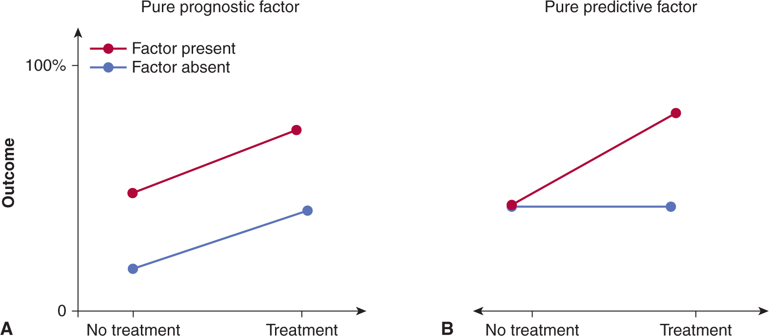
FIGURE 22–10 Differences between prognostic predictive tests. (From Hayes et al, 1998.)

Predictive tests for the selection of cancer drugs are intuitively simple and mirror the routine use of cultures of bacteria causing infections in testing for sensitivity to antibiotics. Testing of anticancer drugs, in which tumor biopsies or cells derived from them are exposed to the drugs in tissue culture, followed by a test that evaluates killing of the tumor cells, has been described for several decades. Initial success was limited, but advances in methods and data acquisition have improved predictive accuracy (Schrag et al, 2004). Despite this, cell-based testing remains a research tool and is not recommended in clinical practice guidelines.

Predictive assays that are in routine clinical use include analysis of estrogen (ER) and/or progesterone receptor (PgR) expression (see Chap. 20, Sec. 20.4.1). This is the most established predictive test in oncology and most oncologists would not consider endocrine therapy for women with breast cancer in the absence of a positive test for tumor cell expression of ER and/or PgR. Another established predictive test is the analysis of HER2 overexpression for the use of trastuzumab or lapatinib. Despite their routine use, validation of these tests is suboptimal. The tests are prone to methodological problems with interobserver and interlaboratory variation occurring in up to 20% of the patients.

More recently, research has focused on predictive factors for activity of inhibitors of the epidermal growth factor receptor (EGFR; see Chap. 7, Sec. 7.5.3 and Chap. 17, Sec. 17.3). The efficacy of drugs targeting the EGFR signaling pathway has been associated with specific mutations in the EGFR gene, increased EGFR gene copy number, absence of K-ras mutations and high expression of genes for endogenous EGFR ligands (Tsao et al, 2005; Lièvre et al, 2006).

Molecular techniques will likely lead to rapid progress in the development of predictive tests. The antitumor activity of an increasing number of targeted therapeutics is based on the presence of specific biomarkers. This has created a need for real-time detection of such genetic aberrations. Some cancer mutations occur at similar DNA bases in tumors from different patients (recurrent mutations). It is therefore possible to use assays that test for single bases (a process referred to as mutation genotyping) to detect these aberrations (Tran et al, 2012). Currently, there are only a few clinically validated recurrent mutations. However, the repertoire of recurrent mutations is increasing, and there is interest in testing these to evaluate their role as predictive mutations for the numerous molecular targeted agents in development. A paradigm shift in the development and use of cancer drugs may be necessary to translate this to patient benefit. Assessment of drug activity in intact tumor cells, and tumor cell gene expression signatures, have potential for the development of versatile predictive tests (Nygren et al, 2008).

22.5 CANCER GENOMICS

The field of cancer genomics is growing rapidly as a result of advances in DNA sequencing technologies (see Chap. 2, Sec. 2.2.10). Two main methods are available to study the cancer genome:

1. Whole-genome sequencing (WGS) is the backbone technology that supports the in-depth sequencing the entire human genome (Metzker, 2009).

2. Targeted genome sequencing refers to strategies that enrich for DNA regions potentially involved in tumor biology. This includes the whole exome or the cancer genome (Robison, 2010).

High-throughput genotyping platforms such as microarrays, have been successfully used for genotyping clinical samples (Thomas et al, 2007). The development of DNA microarray technology holds promise for improvements in the diagnosis, prognosis, and tailoring of treatment. The technical aspects of creating gene expression profiles are described in Chapter 2, Section 2.6. The ability to investigate the transcription of thousands of genes concurrently by using DNA microarrays poses a variety of analytical challenges. Microarray datasets are commonly very large and can be affected by numerous variables. Challenges to microarray analysis include methods for taking into account the effects of background noise (known as normalization of the data), and removal of poor-quality and low-intensity data, as well as choice of a statistical test for determination of significant differences between tumor and control samples (see Chap. 2, Sec. 2.7).

A variety of tests for the identification of statistically significant changes are utilized. These include a spectrum from simple tests such as t-test or analysis of variance (ANOVA), 2 nonparametric smoothing analyses or Bayesian methods. These should be tailored to the specific microarray dataset, and should take into account multiple comparisons. When applied in repeated testing, the standard P-value is conceptually associated with the specificity of a test. Use of a P-value cutoff of less than 0.05 means that false-positive rates will be approximately 5%, but this level of false positivity is too high for microarray data. Consequently, there has been a shift from the use of P-values to the false-discovery rate (FDR; see Chap. 2, Sec. 2.7.2), which is defined as the expected proportion of false positives among the declared significant results.

Cluster analysis is frequently performed to identify genes with similar expression patterns, which are grouped together using either supervised or unsupervised analysis. Supervised analysis involves using samples with 2 or more known characteristics (eg, malignant or benign cells) and developing a gene-expression classification scheme to identify these characteristics. For example, Golub et al (1999), created a classification scheme that was able to distinguish acute myelogenous leukemia from acute lymphoid leukemia based on the expression of 50 genes in 38 samples. This classification method was subsequently able to categorize correctly 29 of 34 test samples. Several alternative methods of classification have been described, including logistic regression, neural networks, and linear discriminant analysis (see Brazma and Vilo, 2000, for explanation of these methods). In unsupervised analysis genes and/or samples with similar properties are clustered together, without reference to predefined sample characteristics. Again, several different algorithms have been developed to perform such cluster analysis. For example, a hierarchical algorithm has been used to cluster different samples of diffuse large B-cell lymphoma with similar gene expression profiles. Two distinct forms with gene expression profiles indicative of different phases of B-cell development were identified. These different clusters could not be identified on the basis of traditional histological features, and could only be distinguished by the gene expression profiles; moreover, the 2 different clusters differed in prognosis (Alizadeh et al, 2000).

The analysis of gene expression profiles is evolving rapidly, and several methodological issues surrounding the use of microarrays in prognostic or other studies are yet to be resolved (see also Chap. 2, Sec 2.7).

1. There is minimal standardization, and researchers have not successfully compared results from different laboratories using different microarray technologies. There is also a lack of rigorous standards for data collection, analysis, and validation.

2. There is little information about measuring the reliability of gene expression levels in microarray experiments. Every measurement has a margin of error. Most clinicians are familiar with the concept of the “confidence interval,” which is used to quantify the uncertainty with which different estimates (eg, of 5-year survival) are made. There are data suggesting that “false-positive” overexpression or “false-negative” underexpression of genes may occur if microarray experiments are not replicated (Ioannidis et al, 2009).

3. DNA microarrays allow one to assess the association between prognosis and the expression of thousands of different genes. The vast amount of DNA expression data obtained from tumor samples from a series of cancer patients virtually ensures that some constellation of gene expression can be found to be associated with prognosis (Petronis, 2010), if that is the goal. Consequently, it is vital that a “prognostic” gene expression profile developed on a training set of tumor samples be validated in an independent and external set of samples to ensure reproducibility of the results.

4. The quality and amount of RNA remains a major challenge in microarray experiments. The amount of tissue obtained and the complexity of the tissue sample can limit the quality and quantity of RNA that can be isolated. Efforts are under way to reduce the amount of sample required for analysis, and newer technologies can analyze samples with only nanogram amounts of tissue.

Related posts:

Chemical Carcinogenesis Tumor Progression and Metastasis Cell Proliferation and Death Drug Resistance Pharmacology of Anticancer Drugs Molecular and Cellular Basis of Radiotherapy

Stay updated, free articles. Join our Telegram channel

Join