Electron-Beam Therapy Dosimetry, Treatment Planning, and Techniques

Eric E. Klein and Rojano Kashani

Megavoltage-photon–based radiation therapy treatment of shallow tumor volumes is complicated by the buildup and radiation transport properties of megavoltage beams. These beams are capable of treating both shallow and deep tumors; however, when treating shallow tumors, the radiation beams transit through the entire patient, exposing distal normal tissues. Megavoltage electron beams have the property of a finite range and therefore do not deliver significant radiation doses to distal depths. Electron-beam therapy is therefore suitable for shallow tumors (<5 cm deep), such as head and neck cancers, skin and lip cancers, chest wall irradiation for breast cancer, and boost dose to nodes. Electrons will typically provide dose uniformity in these target volumes, with minimal dose to distal organs. In fact, G.H. Fletcher¹ had gone as far as saying, “there is no alternative treatment to electron-beam therapy.” Even the strongest proponents of photon or proton therapy acknowledge that electron therapy is necessary to complete any radiotherapy program.

In 1976, Tapley² published one of the earlier comprehensive treatises on electron radiation therapy, in which she states, “There is no practical way for every radiation therapy department, either in hospitals or private offices, to be equipped with all modalities of irradiation beams. Ideally, electron beams should be available for those clinical situations where electrons are indispensable or very clearly superior.” Electrons are now used at most radiation therapy centers. It still might be advantageous to refer patients to regional centers for special treatment techniques utilizing electrons.

Since the late 1970s, there have been three developments in electron-beam radiation therapy technology that have improved significantly our ability to deliver electron therapy. First, the advent of computed tomography (CT)-based treatment planning allowed for coverage of the planning target volume (PTV) by the therapeutic dose and the dose to normal tissues and structures to be more accurately assessed. Use of CT provides a physical description of the anatomy, which is required for accurate dose calculations.^3,4 Second, the development of the electron pencil-beam algorithms (PBAs) and their implementation into treatment-planning systems in the early 1980s provided a mechanism for accurately calculating dose.^5,6 More recently, the use of Monte Carlo calculations has moved development to commercial platforms.⁷ They have demonstrated high degrees of accuracy, especially with the presence of inhomogeneties. Third, manufacturers have refined the quality of their electron beams (i.e., depth dose, off-axis uniformity, and penumbral width) by providing dual-scattering foil systems and electron applicators. Klein et al.⁸ describe dosimetric improvement with the most recent Varian electron-beam delivery system. Presently, the differences in the electron-beam dose characteristics of various radiation therapy machines from different vendors are minimal. More recently, Kashani et al.⁹ described electron-beam characteristics of a new configured beam line in the Varian TrueBeam machine.

Electron-beam therapy is advantageous because it delivers a reasonably uniform dose from the surface to a specific depth, after which dose falls off rapidly, eventually to a near-zero value. The depth of treatment is controlled by selecting the appropriate energy and, when necessary, the bolus thickness. Using electron beams with energies up to 20 MeV allows disease within approximately 6 cm of the surface to be treated effectively, sparing distal normal tissues.

Electron-beam therapy is useful in treating cancer of the skin and lips, upper respiratory and digestive tract, head and neck,^10,11 breast, and a variety of other sites.^2,12,13 Treatment sites of the skin include the eyelids, nose, ear,¹⁴ scalp,^2,15 and more widely spread diseases of the limbs (e.g., melanoma and lymphoma)¹⁶ or total skin (e.g., mycosis fungoides).^17,18 Treatment sites of the upper respiratory and digestive tract include the floor of mouth, soft palate, retromolar trigone, and salivary glands.^10,19 Treatments of the breast include chest wall irradiation following mastectomy^2,20,21; nodal irradiation, often internal mammary chain (IMC) and occasionally axillary; and boost to the surgical bed following mastectomy or lumpectomy.²² Current techniques of using tangential photon adjunct fields abutting supraclavicular and posterior axillary fields are difficult enough without the addition of treating a separate medial breast internal mammary field with a mixture of photon and electrons. Other sites of electron-beam therapy include the retina,²³ orbit,²⁴ paraspinal muscles,^3,25 pancreas and other abdominal structures (intraoperative therapy),²⁶ vulva,²⁷ and cervix (intracavitary irradiation).²⁸

The purpose of this chapter is to discuss the treatment and treatment-planning techniques necessary to deliver the most effective electron-beam therapy. This requires a basic knowledge of dose distribution in water, dose in the heterogeneous patient, treatment-planning tools and principles, and special techniques using electron beams.

DOSE DISTRIBUTION IN WATER

To appreciate the clinical use of electron beams, their dose distributions in water must be understood. Understanding the properties of depth dose, off-axis ratios (OARs), and two-dimensional (2D) isodose contour plots will clarify the concept of dose distribution in water. As well, an understanding of the dependence of the dose distribution on incident energy, field size, and source-to-surface distance (SSD) is required. It is assumed that the dose distribution for a specified energy, field size, and SSD is machine dependent. Applicator design may have a minor influence on dose distributions.

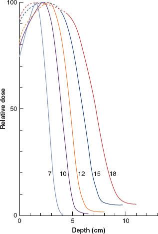
FIGURE 8.1. Energy dependence of depth dose. Plot of relative dose (%) versus depth for a 10 by 10 cm² field size for 7- to 18-MeV beams on a Siemens Mevatron 77 radiation therapy unit (source-to-surface distance, or SSD = 100 cm). (From Meyer JA, Palta JR, Hogstrom KR. Demonstration of relatively new electron dosimetry measurement techniques on the Mevatron 80. Med Phys 1984;11:670–677, with permission.)

Depth Dose

This section discusses percentage of dose (values are normalized to 100% at the depth of dose maximum, R₁₀₀) versus depth in water. Central-axis depth dose implies that the electron field is symmetric about the central axis, and the focus initially will be on square fields. Electron depth dose varies with field size; however, once the field reaches a certain size, side-scatter equilibrium is achieved, and further increasing the size has an insignificant effect on depth dose.^29,30 In the energy range of up to 20 MeV, a 10 by 10 cm² field size typically will achieve side-scatter equilibrium on central axis. The energy dependence of depth dose is illustrated in Figure 8.1, where central-axis depth dose is plotted for a 10 by 10 cm² field for energies in the range of 7 to 18 MeV. The family of curves illustrates how the dosimetric characteristics vary with the incident electron energy:

1. Surface dose (D_s) increases from approximately 75% to 95% as energy increases. The slow increase in dose from the surface to the depth of maximum dose (R₁₀₀) occurs as a result of electrons undergoing multiple Coulomb scattering in water.²⁹

2. Depth of distal 90% (R₉₀), often the therapeutic prescription depth, increases as energy increases.

3. The practical range (R_p) (maximum penetration) of the electrons increases as energy increases.

4. X-ray dose attributable to bremsstrahlung that lies beyond the electron dose component is characterized by its value (D_x) and is taken from the PDD curve 10 cm beyond the practical range (R_p). D_x increases as energy increases. Machines are designed to provide Rx values less than 5%.

5. The R₁₀₀ depth (dmax) can vary irregularly with depth and model of electron treatment machine; its dependence is insignificant for treatment planning, although it is significant to the medical physicist for constructing percent depth–dose data and in beam calibration.

Table 8.1 gives dosimetric parameters for a modern (Triology, Varian) linear accelerator.

TABLE 8.1 VARIAN TRILOGY MEASURED ELECTRON DEPTHS (R_P, R₅₀) AND CALCULATED ENERGIES (E_P, E₀)

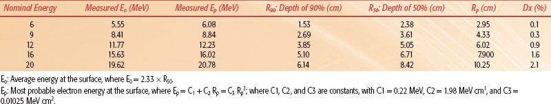
FIGURE 8.2. Field-size dependence of depth dose. Plot of percent dose versus depth for field sizes from 2 by 2 to 25 by 25 cm² for 9-MeV (A) and 20-MeV (B) beams on a Varian Clinac 2100C radiation therapy unit (source-to-surface distance, or SSD = 100 cm).

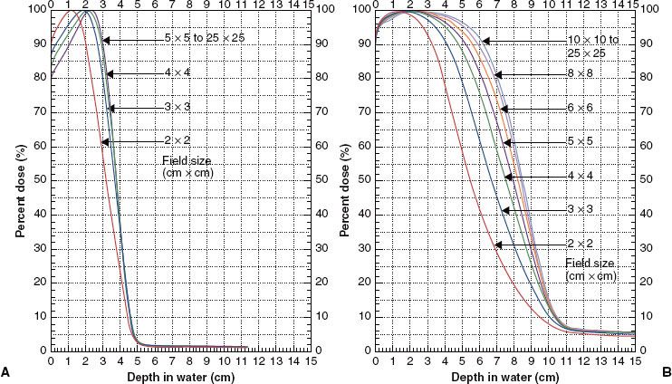
Depth dose has a significant dependence on field size, which varies with incident electron energy. The primary reason for the field-size dependence is loss of side-scatter equilibrium, which has been discussed in detail by Hogstrom²⁹ and Kahn et al.³⁰ Figure 8.2, which shows the field-size dependence of percentage depth dose at 9 and 20 MeV, clearly illustrates that it is a greater issue at higher energies. Loss of side-scatter equilibrium, which begins first at the deeper depths, results in R₉₀ shifting toward the surface as field size decreases. As the field size gets even smaller, the maximum dose decreases, and when it is normalized to 100%, the relative dose at the surface, D_s, increases. In addition, the effects on the distal portion of the depth–dose curve are greater. The most clinically significant effect is the decrease in R₉₀ with decreasing field size, which can require a greater energy than initially proposed for treatment using very small fields (<5 cm).

Depth–dose variations with SSD are usually minimal. Differences in the depth dose resulting from inverse square effect are small because electrons do not penetrate that deep (≤6 cm in the therapeutic region) and because the significant growth of penumbra width with SSD restricts the SSD in clinical practice to typically 115 cm or less. The primary effect of inverse square is that R₉₀ penetrates a few millimeters deeper at extended SSD at the higher energies, as illustrated in Figure 8.3. In relatively few cases (e.g., when the electron beam has a large component of collimator-scattered electrons), the variation in depth dose with SSD can become more significant. In such cases, the collimator-scattered electrons are scattered out of the beam, resulting in a depth dose with a lower D_s and greater R₉₀.³¹

For rectangular fields, Hogstrom³² derived and others have confirmed^31,33 that percentage of depth dose can be calculated by taking the geometric mean of the percentage of depth doses for a square field of length dimension (L) and one of width dimension (W). That is:

If the square field, percentage of depth–dose curves do not have a common R₁₀₀, then the result of equation 1 must be normalized such that its maximum equals 100%. This method is referred to as the square-root method.

In some instances (e.g., intraoperative, intraoral, or intravaginal cones), circular fields are used. In such cases, it will be necessary to measure the dose distributions independent of those determined for square or rectangular fields.

Usually, a collimating insert is placed inside an electron applicator to form an irregular-shaped field, occasionally blocking the central axis. In this instance, central-axis depth dose makes little sense, and the term central-field depth dose should be used, providing that the field has an axis of symmetry. In cases where the insert is irregular, the depth dose can be approximated using a rectangular-shaped field that approximates the irregular-shaped field.³⁴ In highly irregular-shaped fields, the dose distribution should be calculated using an appropriate dose algorithm in a three-dimensional (3D) treatment-planning system. For very small fields, irregular or otherwise, it is highly recommended that PPD measurements be performed to properly determine prescriptive choices (i.e, R₉₀).

FIGURE 8.3. Source-to-surface distance (SSD) dependence of depth dose. Comparison of isodose plots for 15-MeV beam, 10 by 10 cm² at 100-cm SSD with 11 by 11 cm² field at 110-cm SSD. (From Hogstrom KR. Clinical electron-beam dosimetry: basic dosimetry data. In: Purdy JA, ed. Advances in radiation oncology physics: dosimetry, treatment planning, and brachytherapy. Woodbury: American Institute of Physics, 1991:390–429, with permission.)

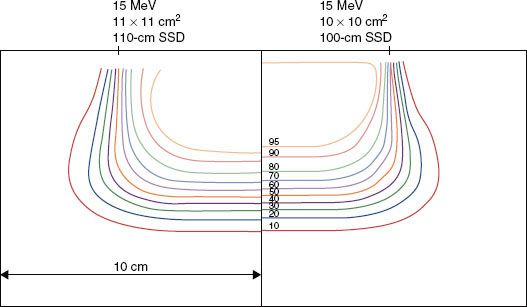
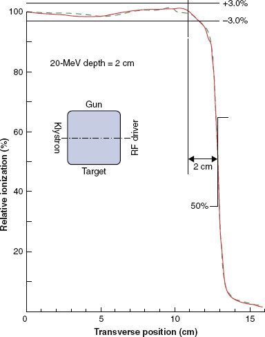
FIGURE 8.4. Beam uniformity verification. Plot of off-axis ratios versus position along a major axis. Data having a negative position (dashed curve) is reflected about central axis for comparison with data having a positive position (solid curve). Data measured at a depth of 2 cm in water at 100-cm SSD for a 20-MeV beam (Varian Clinac 2100C, 25 by 25 cm² open applicator).

Off-Axis Dose

Dose profiles in the dimensions perpendicular to the central axis can be described by OARs. The OAR is defined as the ratio of dose at an off-axis position to that on the central axis at the same depth. OARs measured in water are used to assess off-axis beam quality, which is characterized by flatness and symmetry in the uniform portion of the beam and by its falloff in the region of the penumbra (e.g., 90% to 10%, or 80% to 20%, respectively).

Manufacturers should be able to provide electron beams with a symmetry specification of 2% for opposing points in the beam and a flatness specification of ±3% of the central-axis value along the major axes (±4% along diagonals). The American Association of Physicists in Medicine (AAPM) Task Group 25 recommended that flatness and symmetry should be evaluated along major axes (lines containing central axis and perpendicular to the collimator edges) and along diagonal axes.³⁰ Task Group 25 also recommended that flatness and symmetry be evaluated at depths near the surface and therapeutic depth. Practically, this is performed at R₁₀₀.

Flatness and symmetry are evaluated inside the penumbra, which usually is ensured by setting the boundaries of evaluation 2 cm inside the collimating edge (2√2 cm along diagonals). When physicists acceptance-test a treatment machine, and during subsequent annual reviews, they use the AAPM Task Group 142 recommendations of 2% symmetry and 5% flatness.³⁵ This is usually performed for each energy with an average-size applicator but should be tested for each applicator during acceptance. Subsequently, the profiles acquired during acceptance should be reviewed monthly and be consistent to within 1% of the acceptance values. Figure 8.4 shows the result for a typical accelerator performance evaluation.³⁶

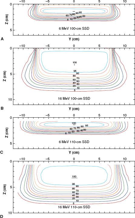
Penumbra of electron beams is predetermined by the design of the beam flattening system, the air gap between the final collimator, and the scatter of electrons in water. Penumbra—a function of depth—is the root mean square addition of two penumbral components: one the result of the air gap and one the result of scatter in the water.⁶ This dependence is complex but can be appreciated qualitatively by the illustration in Figure 8.5, which compares isodose plots for normal (100 cm) and extended (110 cm) SSD at 6 and 16 MeV, respectively. These data show that penumbra grows in a nonlinear fashion with depth, that air gap is more significant at the lower energies, and that scatter in water dominates at the higher energies. Fortunately, the complex dependence of penumbra can be modeled accurately in treatment-planning systems using the pencil-beam or more sophisticated dose algorithms.^29,32,34,37

Isodose Plots

Combining depth dose with OARs results in the 3D dose distribution, and the properties of the 3D dose distribution can be appreciated by viewing 2D isodose contour plots in a plane containing the central axis and a major axis. Examples of these plots for a 15 by 15 cm² field are illustrated in Figure 8.5. As field width decreases or increases, the penumbra shape changes insignificantly because it is most significantly influenced by air gaps and by collimation type. Collimating on the skin, for example, reduces penumbra significantly.

Data required for isodose contours are acquired for an inclusive spread of field sizes at each energy. Two-dimensional isodose contour plots and data are useful for manual treatment planning, input data required by dose algorithms, verification of dose calculated by a treatment-planning system, and quality assurance standards.^29,30,38

FIGURE 8.5. Variation of dose distribution with energy and SSD. Isodose plots (5% to 100%) in water for open 15 by 15 cm² applicator and for 6 MeV, 100-cm SSD (A); 16 MeV, 100-cm SSD (B); 6 MeV, 110-cm SSD (C); and 16 MeV, 110-cm SSD (D) (Varian Clinac 2100C).

DOSE IN THE HETEROGENEOUS PATIENT

For most clinical circumstances, the ideal irradiation condition is for the electron beam to be incident normal to a flat surface with underlying homogeneous soft tissues. The dose distribution for this condition, similar to that for a water phantom described previously, contains a reasonably uniform dose inside the penumbra from the surface to R₉₀, and it has the sharpest possible falloff laterally and with depth. As the angle of incidence deviates from normal, as the surface becomes irregular, and as internal heterogeneous tissues (e.g., air, lung, and bone) become present, the qualities of the dose distribution degrade.³⁹ Internal heterogeneities can change the depth of beam penetration as a result of differences in the rate of energy loss, which can result in PTV underdose and critical structure overdose. Both irregular surfaces and internal heterogeneities create changes in side-scatter equilibrium, producing volumes of increased dose (hot spots) and decreased dose (cold spots), potentially leading to an increased dose to critical structures and decreased dose to the PTV.^3,39 These pertubations can be reduced or eliminated by modifying the treatment technique.

Irregular Surfaces

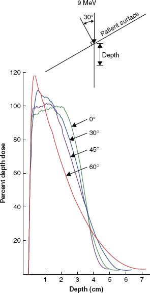
Two geometries that illustrate the effects on the dose distribution caused by an irregular patient surface are the sloped skin surface and the stepped skin surface. Figure 8.6 illustrates changes in the depth–dose curve as a result of nonnormal incidence of an electron beam onto a flat surface. Compared with normal incidence, the nonnormal incident electron beam, central-axis, depth–dose curve shows the following: (a) an increased surface dose, (b) an increased maximum dose, (c) a decreased penetration of the therapeutic dose (R₉₀), and (d) an increased range of penetration.^30,40 These changes can be clinically significant, particularly at angles of incidence greater than 30 degrees from the normal. Such conditions can occur when irradiating curved patient surfaces with large fields (e.g., chest wall, limbs, neck, and scalp). In addition, it should be appreciated that the depth of R₉₀ is specified along the central axis of the beam, and if the depth is taken perpendicular to the surface, then the depth is further reduced (approximately) by a factor cos (φ), where φ is the deviation of the incident angle from the normal.

Any time a sharp gradient (stepped surface) occurs on the patient’s surface, side-scatter equilibrium will be lost, resulting in a cold spot beneath the proximal surface and a hot spot beneath the distal surface.^32,39,41,42 This can occur as a result of a sharp bolus edge, surgical defects, or within normal anatomy. For example, in the use of a uniform thickness bolus that partially covers a field, a 90-degree step can result in hot or cold spots as great as 20%, as illustrated in Figure 8.7. In such a case, the bolus should be tapered as much as possible. The results of a 45-degree tapered bolus in Figure 8.7 show a reduction in the hot spot but, more significantly, an increased coverage of the 90% isodose contour. The nose is a protrusion that creates a cold spot beneath itself, often the location of the tumor.^5,33,39 The ear canal (Fig. 8.8) and surgical voids, which are characterized by a depression in the patient’s surface, can result in hot spots in excess of 50%, depending on void dimension and beam energy.^43,44 Such depressions normally should be filled with some type of bolus material. Normal anatomy contains many irregular surface depressions and protrusions (e.g., the ear canal and the nose, respectively) and should be accounted for by accurate treatment planning.

FIGURE 8.6. Effect of angle of incidence on depth dose. Dose versus depth for a 9-MeV beam incident on water angled 0 degrees to 60 degrees from the normal. (From Ekstrand KE, Dixon RL. The problem of obliquely incident beams in electron-beam treatment planning. Med Phys 1982;9:276–278, with permission.)

Air Cavities

The influence of an internal air cavity is illustrated in Figure 8.9, which compares isodose contours beneath an air cavity to those without the air cavity. Results show that (a) the isodose contours in the shadow of air are shifted distally, (b) the dose beneath the air cavity increases as a result of loss of side-scatter equilibrium, and (c) the influence of the air increases laterally with depth. Internal air cavities of clinical interest primarily occur in treatment of the head and neck (e.g., nasal passages, ethmoid sinuses, maxillary sinuses, larynx, and mastoids).^32,39

Another significant effect is the reduction in dose in unit density tissue lateral to an air cavity. Electrons scattering from the unit density tissue into the air are not replaced because air is unable to scatter an equal amount back into the unit density tissue. Frequently, nose tumors can spread into the septum, in which case bolus should be used to eliminate or reduce underdosing.

Lung

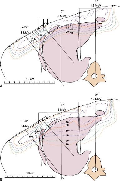
In lung, electrons can penetrate three to four times farther than in unit density tissue. This is demonstrated in Figure 8.10, where isodose contours from a typical electron chest wall treatment are compared with those in which the lung is assumed unit density. Assuming a given dose of 50 Gy, the 40% isodose contour corresponds to 20 Gy, approximately the threshold for pneumonitis, if significant lung volume is irradiated. Ignoring the low density of lung would grossly underestimate the volume of lung receiving more than 20 Gy.³²

This effect increases with energy. For example, increasing the beam energy from 9 to 12 MeV results in an additional 1.5 cm of penetration in waterlike tissue (electrons lose energy at a rate of approximately 2 MeV per centimeter in water), and this corresponds to as much as 6.0 cm in lung (assuming a lung density of 25%). Consider the patient whose chest wall thickness requires an energy of 10 MeV for treatment and that 12 MeV must be selected. This results in as much as 4 cm in depth of needless irradiation in lung, unless 1 cm of bolus is used to effectively lower the energy incident on the patient to 10 MeV.

Care must be taken when irradiating targets where the lung is immediately distal, such as with entire chest wall irradiation.

Bone

Interactions of electrons with bone are complex and interesting. The influence of bone is illustrated in Figure 8.11, which compares isodose contours beneath hard bone to those without the bone. The results show that:

1. The isodose contours in the shadow of the bone are shifted proximally,

2. Dose outside (inside) the bone–water interface increases (decreases) by approximately 5% as a result of loss of side-scatter equilibrium, and

3. The lateral dimension of the region having its dose perturbed by the bone increases with depth.

Actual bones are not uniformly dense throughout their cross-section, and in most cases their edges are not parallel to the incident beam. Both differences decrease the influence of bone in generating inhomogeneity in the patient’s dose distribution. Dense bones that significantly affect the dose distribution include the mandible, bones of the skull (e.g., frontal bone and zygoma in orbit treatment or temporal bone in treatment of parotid), clavicles, and vertebral processes (e.g., craniospinal irradiation).

One might ask, what is the clinical significance of the increase in dose in or around bone due to increased scatter? The maximum dose increase expected as a result of backscattered electrons is 5%, and the maximum dose increase expected inside bone and in adjacent exit tissues is approximately 7%.⁴⁵ These increases represent maximum dose estimates because actual bones are not as dense through and through as are the bone substitute in which these data were taken. These estimates of the increased dose are not expected to be clinically significant. In fact, untoward effects in or around bone that can be attributed to dosimetry have not been observed in patients treated with electron-beam therapy.

FIGURE 8.7. Effect of irregular patient surface on dose distribution. Plot of isodose contours for a 12-MeV, 15 by 15 cm² beam incident on water at 100-cm source-to-surface distance (SSD) having a stepped surface resulting from a 2-cm slab of bolus (A) and a beveled edge (45 degree) on the stepped surface (B). The dashed line in the top figure shows the location of the 90% isodose contour in the bottom one. (From Hogstrom KR. Treatment planning in electron-beam therapy. In: Vaeth JM, Meyer JL, eds. Frontiers of radiation therapy and oncology vol. 25: the role of high energy electrons in the treatment of cancer. Basel: S. Karger AG, 1991:30–52, with permission.)

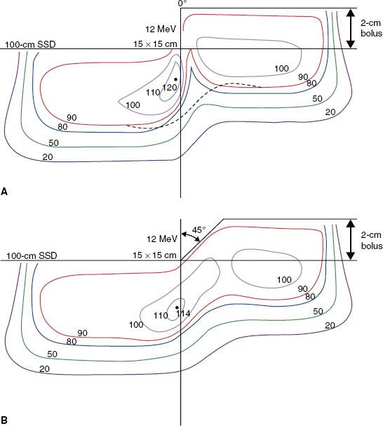
FIGURE 8.8. Impact of irregular surface anatomy on dose distribution. A 15-MeV electron beam irradiates the left side of a patient treated for dermal squamous carcinoma with perineural invasion. A beeswax bolus protects the posterior cranial fossa and the maxillary sinus. Isodose contours, expressed as a percentage of given dose, show how the ear canal results in an unacceptable hot spot of 160% to the middle ear (A) and how filling the ear canal with bolus (saline solution) eliminates that hot spot (B). The residual hot spot of 125% is a result of the external ear. (From Morrison WH, Wong PF, Starkschall G, et al. Water bolus for electron irradiation of the ear canal. Int J Radiat Oncol Biol Phys 1995;33:479–483, with permission.)

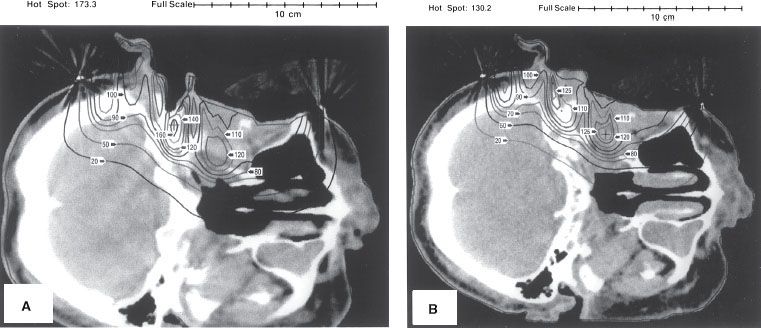
FIGURE 8.9. Effect of internal air cavity on underlying dose distribution. Dose calculated by the pencil-beam algorithm (PBA) for a 2 by 2 cm² cylinder of air located 2 cm below the surface in water is compared to that in its absence. (From Hogstrom KR. Dosimetry of electron heterogeneities. In: Wright AE, Boyer AL, eds. Advances in radiation therapy treatment planning. New York: American Institute of Physics, 1983:223–243, with permission.)

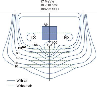
FIGURE 8.10. Effect of lung on dose distribution underlying chest wall. Comparison of dose calculated by the pencil-beam algorithm (PBA) for 8-MeV chest wall irradiation, assuming patient is water (A) and heterogeneous anatomy (B) based on computed tomography data.

DOSE PRESCRIPTION AND CALCULATION OF MONITOR UNITS

Dose Prescription

It is recommended that dose be prescribed to given dose or 90% of given dose. Intermediate or lower prescription (95%, 85%, 80%) can be prescribed if the energy (typically stepped in 3 to 4 MeV increments) choices are too coarse to maintain a single baseline prescription recipe. Given dose is defined as the maximum central-axis dose in a water phantom at the SSD of the patient for the energy, applicator, and field size identical to that used for patient treatment. If the field shape is irregular, then the field size is taken to be a rectangular field representative of the irregular field shape. The most representative rectangular field is not well defined; however, Hogstrom et al.³⁷ have provided one methodology for determining its estimate.

It is recommended that dose be prescribed to given dose or a percentage of it and not to a point in the patient. It is quite possible that a dose prescription point in the patient could be in a region of increased or decreased dose because of tissue heterogeneity or irregular surface, which could result in PTV underdose or overdose, respectively.

Calculation of Monitor Units

Monitor units can be determined by

where D_prescribed is the prescribed dose, %D is the percentage of given dose to which dose is prescribed (e.g., 90%), and O(E, C, LxW, SSD) is the output (dose per monitor unit) for a beam of energy E, applicator C, field size LxW, and SSD. To use this methodology, the medical physicist must measure dose output as a function of square field size and SSD for each energy-applicator combination at the time of commissioning the accelerator. Output for rectangular fields can be determined using the square-root method of Mills et al.^14,46 and Shiu et al.³¹:

Output for rectangular fields also can be determined using an equivalent square method^30,33,47,48; however, Biggs et al.⁴⁷ recommend limiting this method to an aspect ratio (L:W) of 2:1. The square-root method is not limited to the aspect ratio, and Shiu et al.³¹ have shown it to be more accurate. Figure 8.12 illustrates beam output data at 9 MeV for four common applicators used on the Varian Clinac 2100C (Varian Medical Systems, Palo Alto, CA) at 100 cm SSD.

Output at extended SSD can be determined by either the air-gap method or the effective-source method.³⁰ The effective-source method is covered in detail by Khan.⁴⁸ The air-gap method has a sounder physical basis. Although both methods give similar answers, only the air-gap method will be covered here.³³ Output at extended SSD is given by the product of output at the nominal SSD (SSD₀), the air-gap factor (fair), and an inverse square term,

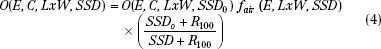
f_air is determined by measuring dose output for square fields at the extended SSD and then solving equation 4. For rectangular fields, the air-gap factor is determined using the square-root method³¹:

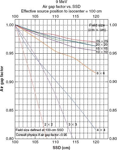
As f_air is assumed independent of applicator, the dose output needs to be measured only for the smallest applicator that contains the square field size. Figure 8.13 plots the square field air-gap factors for the 9-MeV beam of the Varian Clinac 2100C for SSD from 100 to 120 cm. For a more detailed explanation of dose output and sample calculations of monitor units for electron beams, refer to Hogstrom et al.³⁴ Another practical option is to fix incremented SSDs to be used clinically (i.e., 100, 105, 110, 115 cm) and establish tabular outputs for each energy/applicator SSD combination.

FIGURE 8.11. Effect of hard bone on underlying dose distribution. Dose calculated by the pencil-beam algorithm (PBA) for a 3 by 1 cm² cylinder of hard bone substitute located 1 cm below the surface in water is compared to that in its absence. (From Hogstrom KR. Dosimetry of electron heterogeneities. In: Wright AE, Boyer AL, eds. Advances in radiation therapy treatment planning. New York: American Institute of Physics, 1983:223–243, with permission.)

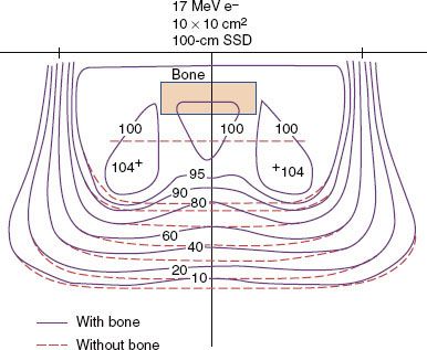
FIGURE 8.12. Field-size dependence of output (dose/monitor unit). Plot of output factor (cGy/MU) versus side of square field from 2 by 2 cm² to the open applicator for four applicators and for the 9-MeV beam of a Varian Clinac 2100C.

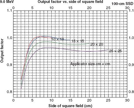
FIGURE 8.13. Dependence of air-gap factors on source-to-surface distance (SSD) and field size. Plot of f_air versus SSD for field sizes ranging from 2 by 2 to 25 by 25 cm² and for the 9-MeV beam (Varian Clinac 2100C).

CALCULATION OF DOSE IN PATIENT

Standards for Patient Dose Calculations

Sound treatment-planning decisions require accurate dose calculation in the patient. Therefore, the following recommendations are made for electron-beam treatment planning. First, dose should be calculated in the full three dimensions to allow for evaluation of dose homogeneity in the PTV, coverage of the PTV by the 90% isodose contour, and dose to critical structures. Second, the dose algorithm should account for patient heterogeneity. Failure to properly account for patient heterogeneity can result in failure to appreciate dose heterogeneity, PTV underdose, or normal-tissue overdose.^5,39,49 Third, the dose algorithm should be accurate, and for those conditions for which this is not the case, physicians and physicists should discuss the proper interpretation of the dose calculations.

To expand on the final recommendation, a dose algorithm must meet certain criteria to be most effective in the clinic.⁵⁰ First, it should be accurate to within 4% in regions of low-dose gradients or within 2 mm in regions of high-dose gradient (e.g., penumbra or depth-dose falloff region).^38,51 Second, the dose algorithm should be commissioned easily by a qualified medical physicist. Third, the accuracy of the dose algorithm should be well documented. Since 1981, the PBA has best met this requirement. Presently, several new, more accurate algorithms, both analytical and Monte Carlo–based, are being implemented into commercial treatment-planning systems and will replace or supplement the PBA in due time.⁵² Regardless of the algorithm, it is the medical physicist’s responsibility to commission the algorithm, to understand its accuracy, and to train medical dosimetrists and radiation oncologists in its use and limitations.

Dose Algorithms

For the past 20 years, the standard methodology for dose calculation in the patient has been the PBA. As computing power increased, it was possible to implement the algorithms into 3D format.⁵³ Detailed instructions for commissioning the dose algorithm and documentation of its accuracy have been published.^5,6,50 The PBA has been shown to be quite accurate in water at standard and extended SSD, correctly predicting the changes in penumbra.^29,32,34 It is also quite accurate in predicting changes in dose resulting from oblique incidence and irregular surfaces.^5,50 Regarding internal heterogeneities, it correctly predicts the penetration in lung and the growth of the penumbra width in lung⁵⁰; however, it tends to underestimate the dose in lung near the mediastinum as a result of its central axis approximation.⁵⁰ In bone, it correctly predicts the shortening of the dose penetration behind the bone, and it slightly underestimates (<5%) the magnitude of the hot and cold spots under the edge of a thick hard bone such as the mandible.⁵ The PBA does not predict the increased dose (<5%) resulting from backscatter at the proximal tissue–bone interface, nor does it predict the increased dose (>7%) in bone resulting from increased scatter. The PBA underestimates the hot and cold spots under the air–tissue interfaces.^5,50

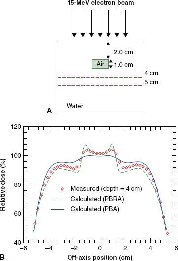
New dose algorithms that are accurate to 4% or better are becoming available in commercial treatment-planning systems. Many of these algorithms have been reviewed by Hogstrom and Steadham.⁵⁰ One of these is the pencil-beam redefinition algorithm (PBRA), whose commissioning is similar to that of the conventional PBA, although its accuracy is significantly improved.^54–56 Figure 8.14 illustrates the improvement of the PBRA.

Many of the newer algorithms are based on Monte Carlo methods, which allow them to be quite accurate.^57–61 Cygler et al.⁵² published a report on the first commercial system using Monte Carlo–based electron calculations, demonstrating excellent results. Ding et al.⁶² demonstrated outstanding results for a macro–Monte Carlo algorithm, along with a companion report showing superior results for Monte Carlo compared with PBA.⁶³

FIGURE 8.14. Evaluation of accuracy of dose algorithms below air cavity. A: Dose is measured distal to an internal air cavity. B: Measured dose profile at a depth of 4 cm is compared to that calculated by the pencil-beam algorithm and the pencil-beam redefinition algorithm. PBA, pencil-beam algorithm; PRBA, pencil-beam redefinition algorithm. (From Shiu AS, Hogstrom KR. Pencil-beam redefinition algorithm for electron dose distributions. Med Phys 1991;18:7–18, with permission.)