Fig. 3.1
Expression profiling schema. Above, schematic depiction of two-color hybridization on cDNA or oligonucleotide microarrays. RNA isolated from test and reference samples is labeled with two different fluors (here pseudocolored red and green), then co-hybridized to the array. For each gene on the array, the ratio of red/green fluorescence (typically reported in log2 scale) reflects its relative transcript abundance in the test compared to reference sample. Below, schematic depiction of one-color hybridization on Affymetrix GeneChip oligonucleotide arrays. RNA is biotin-labeled by in vitro transcription (IVT), then hybridized to the array. Multiple different probes report on each gene, where expression levels can be represented by the difference in average staining intensity between perfect match (PM) and control mismatch (MM) probes.
Experiments using Affymetrix GeneChip arrays , in contrast, are carried out as one-color hybridizations (Fig. 3.1). A single RNA sample is labeled by cDNA synthesis, using an oligo(dT) primer with a T7 RNA polymerase promoter site, followed by in vitro transcription in the presence of biotinylated nucleotides. The resultant biotinylated antisense RNA targets are then fragmented and hybridized to the microarray, where they bind to their cognate sense oligonucleotide probes. Following washing, a streptavidin–phycoerythrin fluorophore conjugate is used to stain bound target which is then visualized by fluorescence scanning. For each gene represented on the array, the fluorescence intensity reflects that gene’s level of expression in the labeled sample.
3.2.3 Experimental Design Considerations
For experiments comparing test and reference samples, a two-color microarray platform provides a more direct comparison. Examples of such studies include treatment (e.g., drug or siRNA) versus control, tumor versus matched normal, or time course experiments where the zero time point is a natural reference. For studies profiling collections of tumors there is no such natural reference, but a universal reference RNA, e.g., comprising pooled RNA from a set of tumor-derived cell lines, can be used [4]. Since all tumor samples are hybridized against the same reference RNA, tumor gene-expression ratios share the same denominator and can be compared amongst one another [5]. For tumor profiling studies, a single-color microarray platform obviates the need for a reference RNA.
Like any other assay, microarray results need to be reproducible. Technical replicates, where the same sample is labeled and hybridized again, can be used to verify measurements. Dye-swap experiments, where for two-color hybridizations the fluorophores used to label the test and reference sample are interchanged, serve as a control for possible dye-labeling bias. Biological replicates, in which the experimental samples are themselves recreated, and then labeled and hybridized, provide the greatest measure of reproducibility, controlling for biological as well as technical variation [6]. However, for exploratory profiling studies, assaying additional cancer samples may generate greater depth of information than assaying fewer samples, but in replicate. Microarray results, at least for key genes, are often verified using independent assays. Such technical validation might include Northern blot or quantitative reverse-transcription PCR (qPCR). Using a second, different microarray platform can serve to verify measurements for many genes at once.
A goal of expression profiling studies is often to identify genes differentially expressed between two groups. Because such studies are exploratory, it is difficult to estimate the number of samples needed. Analysis of existing datasets indicates that at least five samples from each group are needed [7]. However, reason would dictate that the more similar the sample groups are to one another, the larger the number of samples would need to be profiled to identify significant expression differences.
3.2.4 Specimen Considerations
Common epithelial cancer types are heterogeneous at the tissue level, composed of varying fractions of neoplastic cells, normal epithelial cells, and tumor stroma, including fibroblasts, endothelial cells, and various immune cells. Even different parts of the same cancer may vary in these cell fractions. Studies using undissected cancer tissues should be interpreted with this cellular heterogeneity in mind. Microdissection techniques , including laser capture microdissection [8], can be used to obtain and profile specific tissue compartments like cancer epithelium. Alternatively, computational methods can be used for in silico dissection of whole cancers, where for example specific gene-expression patterns are attributed to cell types by comparison to expression patterns of cognate cultured cells [9], or by correlating patterns with cell fractions observed histologically [10].
Conventional RNA labeling methods require microgram quantities of input RNA. However, microdissected specimens typically yield only nanogram amounts. Protocols are available to amplify the input RNA. A common method of linear amplification, better preserving relative transcript abundances, makes use of in vitro transcription [11]. Alternatively, signal amplification can be used to augment the hybridization signal from low amounts of input RNA [12]. While fresh or freshly frozen specimens provide the highest quality RNA for microarray analysis, some success has been reported in extracting usable RNA from formalin-fixed paraffin-embedded (FFPE) specimens [13, 14], which are more readily available from pathology archives.
3.3 Analysis of Expression Profiling Data
3.3.1 Data Processing
After imaging the hybridized microarray, feature extraction (spot finding) software is used to locate DNA features on the microarray, and to associate annotated probe features with fluorescence intensity measurements. For two-color hybridizations on spotted DNA microarrays, background fluorescence intensity surrounding spot features is typically subtracted out to better estimate specific hybridization signal. For each gene spot, fluorescence intensities for the two colors are next converted to a single fluorescence ratio, which describes the relative expression of the corresponding gene between the two samples. By converting fluorescence intensities to ratios, information on the absolute level of expression is lost, but might be inaccurate anyway due to variation in the amount of spotted DNA probe. Fluorescence ratios are then converted to log ratios, most often using log2 values. In log space, increased and decreased expression is mathematically symmetric with opposite signs (while in linear space decreased expression is compressed within ratios between 0 and 1).
For Affymetrix GeneChip arrays , where a set of DNA oligonucleotide probes is used to report on each gene, fluorescence intensities are calculated as the mean intensity for the probe set. Nonspecific hybridization, calculated from the mean intensity of a matched set of oligonucleotide probes containing a single central nucleotide mismatch, can be subtracted out to yield an average difference. While fluorescence intensities bear some relation to absolute expression levels, target amplification is inherent in the labeling protocol and can bias transcript representation. Therefore, log intensities are typically converted to ratios as described further below.
Once fluorescence signals are extracted, the data need to be normalized to compensate for any differences in the amount of input RNA, or in the labeling or detection efficiency occurring either between two samples on the same array, or between samples on different arrays [15]. For two-color microarray hybridizations, global normalization entails scaling intensities such that the sum of all gene intensities for the two fluorescence channels is set equal (which is equivalent to scaling the average log ratio to zero). Lowess normalization can also correct for signal intensity-dependent dye biases [15]. Another approach is to use the so-called house-keeping genes, those whose expression is most invariant across samples, to normalize ratios between different samples. Likewise for Affymetrix arrays, normalization between different arrays can be accomplished by scaling intensities globally or by using housekeeping genes.
In addition to array normalization, another common data transformation is mean centering genes across a set of array hybridizations. This transformation is often applied to two-color microarray datasets such as tumor profiling studies where a universal reference RNA is used. For each gene in each sample, the log fluorescence ratio is mean centered by subtracting that gene’s average log fluorescence ratio for the sample set. The result is that fluorescence ratios reflect gene expression levels in relation to the sample set average, rather than to the arbitrary universal reference. For Affymetrix datasets, log intensities for each gene are often converted to log pseudo-ratios by subtracting the average log intensity for that gene in the sample set, which in effect centers genes.
The quality of a microarray hybridization can be assessed using external spike-in controls (e.g., bacterial transcripts, with cognate probes on the array), where observed and expected fluorescence ratios can be compared. In addition, replicate features on the microarray can provide a measure of intra-array reproducibility indicative of performance. Ultimately, raw and processed microarray data files, along with annotations compliant with minimal information about a microarray experiment (MIAME) standards [16], can be deposited into a public repository like GEO [17] or ArrayExpress [18].
3.3.2 Visualizing Data
Whichever microarray platform is used, the end result of a set of array hybridizations can be summarized in a table (or matrix) of gene expression values (typically ratios) (Fig. 3.2). Each row of the table corresponds to a different gene probe on the array, each column corresponds to a different arrayed sample, and each entry in the table represents the expression level of a particular gene for a particular sample. To more readily discern patterns in the data, these numeric tables are typically visualized as colorimetric tables, or heatmaps, where expression levels are represented with a color scale (Fig. 3.2). Common colorimetric representations include red/green (or red/blue) for increased and decreased expression, respectively. Several software tools are available to process, visualize and/or perform basic analyses of microarray data, from academic (Stanford Microarray Database [19]), government (BRB-ArrayTools [20]), and commercial sources (GeneSpring, SpotFire, and Oncomine [21, 22]).
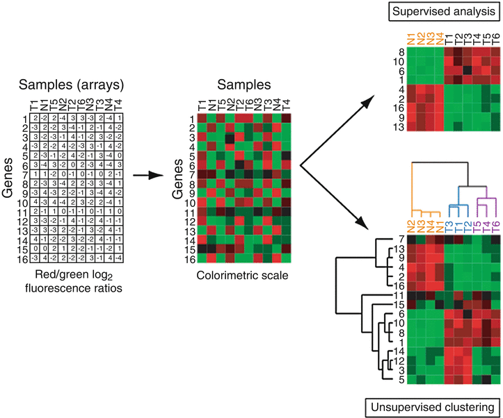

Fig. 3.2
Microarray data analysis. Left, the starting point of microarray analysis is a matrix of gene expression ratios, where each row is a different gene and each column is a different sample (array). Center, viewing ratios in colorimetric scale facilitates recognition of expression patterns. Above right, analysis supervised on the tumor (T) versus normal (N) distinction identifies the subset of genes with significant differences in expression, here ranked by t-statistic. Below right, hierarchical clustering analysis of the same input data matrix reveals the tumor-normal distinction, but also suggests the presence of two tumor subclasses (highlighted by blue and purple dendrogram branches).
3.3.3 Analyzing Data
Microarray data are often filtered prior to analysis. For example, genes whose expression varies little across the sample set can be excluded from subsequent analysis, using ratio-fold or standard deviation cutoffs. Such data filtering can increase the subsequent yield of significant genes (by reducing the total number of genes tested), though also represents a source of variable findings among different microarray studies.
Analysis of microarray data can be broadly divided into two approaches, supervised and unsupervised [23, 24]. Supervised methods make up-front use of specimen information, for example to identify genes differentially expressed between two different specimen classes such as cancer and normal (Fig. 3.2). Various metrics can be used, like ratio-fold difference, or the Student’s t-statistic which highlights genes with a large between-class difference in average expression compared to within-class expression variance. While metrics like the t-statistic provide an associated P-value, it is important to correct for multiple hypothesis (gene) testing (discussed more below). The number of truly (and falsely) significant genes can be estimated by comparing the number of genes observed (at any given threshold) in the real data to the median number observed in many samplings of randomly permuted data, generated for example by shuffling the sample class (e.g., cancer versus normal) labels. Significance Analysis of Microarrays (SAM) is a commonly used analysis software tool that provides such false discovery rate estimates [25].
Genes differentially expressed between sample classes can provide a basis to classify new samples. There are different methods for classifying samples, including weighted voting [26] and Prediction Analysis of Microarrays (PAM) , based on nearest shrunken centroids [27]. Though the specifics differ, the principle is to determine whether the expression of classifier genes in a new sample better matches that of one or the other known sample classes used to develop (or train) the classifier. The new sample is assigned to the class with the better match, and the confidence of that assignment can be summarized as the strength of the prediction for one class over the other. The overall performance of a classifier can be estimated in the training set (where classes are known) by leave-one-out cross-validation (LOOCV), wherein one sample is omitted and a classifier is trained on the remaining samples and tested by predicting the class of the omitted sample. The process is repeated leaving a different sample out each time, and performance is then summarized by the overall classification accuracy on all samples. Classifier performance should also be validated by analyzing a separate test sample set that is independent of the training set.
In contrast to supervised approaches, unsupervised methods organize data agnostic to information about the samples, and are therefore useful for discovering previously unknown relationships in the data. Hierarchical clustering analysis is one such widely used unsupervised method [28] (Fig. 3.2). In hierarchical clustering, an iterative agglomerative algorithm is used to reorder the rows (genes) and columns (arrayed samples) of the expression matrix such that genes with similar vectors of expression across the samples (e.g., by Pearson correlation) are clustered (or grouped) together, and, independently, samples with similar vectors of expression across the genes are clustered together. Analogous to phylogenetic analysis, dendrograms (or trees) display the hierarchical relationships among genes and among samples, and the reordered heatmap highlights prominent patterns of gene expression. Information about the samples and genes can then be overlaid on the dendrograms to assist in interpreting patterns of expression. Such clustered heatmaps have been likened to molecular portraits [9], and provide a powerful new approach to observe, describe, and understand the molecular variation within cancer specimens, and in particular to discover previously unrecognized cancer subtypes.
Another useful way to organize and view microarray data, and to interpret expression patterns identified from supervised or unsupervised analysis, is pathway (or network) analysis. Gene ontology (GO) terms categorize genes by cellular component, biological process and molecular function [29]. Likewise, database resources like BioCarta and the Kyoto Encyclopedia of Genes and Genomes (KEGG) [30] place genes in biological pathways (e.g., metabolic and signal transduction pathways) [31]. Finding statistical enrichment of specific GO terms or cellular pathways can suggest biological meaning for a group of genes of interest. Another related approach is gene set enrichment analysis (GSEA) , which evaluates enrichment for each of several hundred curated gene sets by determining their overrepresentation at the top of a list of genes rank ordered by their expression distinction between two sample classes [32]. The gene sets include groupings from biological pathway databases, as well as groups with shared expression (from published microarray studies), promoter regulatory motifs, or cytogenetic location. Related methods can be used to assess enrichment of interactive networks of genes [Ingenuity Pathways Analysis—http://www.ingenuity.com/] or molecular concepts [33].
3.3.4 Common Pitfalls in Data Analysis
In profiling across many genes and specimens, the resultant high-dimensional microarray datasets have brought new statistical challenges [6, 34]. A common pitfall is reporting significant differentially expressed genes without having corrected for multiple gene testing. In large datasets, almost any particular expression pattern sought can be found, but may not be statistically meaningful. For example, in identifying genes differentially expressed between cancer and normal tissue from a dataset of 10,000 genes, about 500 genes would be expected to have individual P-values of less than 0.05 (the standard threshold of statistical significance) just by chance! True statistical significance is best assessed by comparison of observed findings to those from randomly permuted data.
Another common pitfall is over-fitting the data, where data models (like classifiers or outcome predictors) are developed and then tested on the exact same samples, rather than on an independent sample set. The result is an inflated estimate of test performance. An additional common shortcoming is the use of insufficiently large sample sets in both training and validation phases of analysis. Early microarray studies using inappropriate statistical methods likely contributed to overly inflated expectations of the technology.
3.4 Expression Profiling—Applications
3.4.1 Cancer Classification
A major goal of many DNA microarray studies is cancer classification . Cancers are classified principally based on their tissue of origin and histology, and sometimes with the aid of ancillary tests like immunohistochemistry, flow cytometry, and cytogenetics. Classification schemes provide important information for prognostication and for the selection of optimal therapies. Much as the pathologist uses histologic patterns to classify cancers, DNA microarrays describe patterns of molecular variation, hitherto unrecognized, having the potential to improve cancer classification.
In an early landmark study, Golub et al. [26] described the computational framework for applying DNA microarrays to the problem of cancer classification. Using supervised methods, the investigators identified genes differentially expressed between two classes of leukemia, acute myelogenous leukemia (AML) and acute lymphoblastic leukemia (ALL). Statistically significant differences could be defined as those occurring above what was expected by chance, estimated by comparison to randomly permuted data. Using the top-most significant genes, a classifier could be developed that accurately predicted the diagnosis of new cases. While AML and ALL are in reality readily distinguishable by existing cytochemical staining and flow cytometry techniques, the concepts developed, and many variations on the original computational methods, are applicable to more challenging classification problems.
One such classification problem currently receiving attention is that of metastatic cancers of unknown primary (CUP), which account for up to 5 % of newly diagnosed cancers [35]. Despite subsequent immunohistochemical staining and imaging studies (like computed tomography), the anatomic site and tissue of origin remains undetermined in many cases, where knowing that information is important for selecting the optimal treatment regimen [36]. DNA microarrays have been used to define cancer type-specific patterns of gene expression, which have been shown to classify new cancer cases (where clinical truth is known) with ~80–90 % accuracy [37–40].
3.4.2 Cancer Class Discovery
Another important application of DNA microarrays is the discovery of new, previously unrecognized tumor classes, as first reported by Alizadeh et al. [41]. By unsupervised cluster analysis of variably expressed genes, these investigators identified two subtypes of diffuse large B-cell lymphoma (DLBCL) with distinct expression patterns. One pattern shared similarities with normal germinal center B cells, while the other with activated B cells. The latter DLBCL subtype was also associated with constitutive NFκB activity and less favorable prognosis [41, 42]. Therefore, while indistinguishable by histology, expression profiling nonetheless suggested a refined classification of DLBCL that might improve outcome prediction and possibly selection of therapies. Indeed, BCL6 gene expression, a surrogate indicator of the germinal center B cell-like subtype, has since been shown to predict survival independently of the currently used International Prognostic Index score [43].
Microarray analysis of breast cancer has also identified multiple tumor subclasses, refining the existing classification [9, 44]. Estrogen receptor (ER)-positive breast tumors could be subdivided into two luminal subtypes (called so because of shared expression markers with the luminal layer of normal breast epithelium), luminal A and B, with the latter associated with higher proliferation rates and less favorable outcome. ER-negative tumors included those with ERBB2 (Her2/neu) amplification as well as a previously underappreciated basal-like subtype (with shared expression markers of the basal/myoepithelial layer of normal breast epithelial) with poor prognosis. Similar microarray studies have identified tumor subclasses within other tumor types as well [45].
3.4.3 Outcome Prediction
Microarray analysis has also been applied to directly define gene signatures for prognostication and for prediction of response to therapies. In a seminal study, van’t Veer et al. [46] compared gene-expression profiles of breast cancers from women who either did or did not develop distant metastases within 5 years of follow-up. Supervised analysis defined a 70-gene signature that could predict disease-free and overall survival in an independent cohort of breast cancer patients [47], outperforming current prognostic indices based on clinical and histological parameters such as the St. Galen and NIH consensus criteria [48]. The poor-prognosis signature might therefore improve the selection of patients who would benefit from adjuvant therapy. Prognostic and predictive signatures have been proposed for other cancer types as well, including a 133-gene prognostic signature in AML [49], independently validated [50] and with potential utility in risk-stratification for cases with normal cytogenetics.
3.4.4 Biological Insight
Expression profiling has made many other significant contributions to our understanding of cancer biology. For example, Ramaswamy et al. [51] explored gene expression differences between unmatched primary and metastatic adenocarcinomas of diverse tumor types. The investigators defined a 17-gene signature of metastasis which, unexpectedly, was also expressed in a subset of primary tumors where its presence predicted metastasis and poor clinical outcome. Importantly, this study challenged the existing paradigm that metastases arise from rare cells in the primary tumor that have acquired additional genetic alterations, suggesting rather that the propensity to metastasize characterizes the bulk population of tumor cells, and therefore by inference is determined early in tumor development.
Another seminal contribution of microarray analysis was the relatively recent discovery of recurrent gene fusions in prostate cancer. By analyzing outlier values of gene expression in microarray datasets, Tomlins et al. [52] identified elevated expression of ERG and ETV1 (oncogenic ETS family transcriptional factors) in subsets of prostate cancer. Further characterization revealed chromosome rearrangement and gene fusion, resulting in the promoter of the androgen-regulated gene TMPRSS2 driving overexpression of ERG or ETV1. This finding provides novel insight into androgen-dependent prostate tumorigenesis, and challenges the longstanding assumption that recurrent chromosomal rearrangements, frequent in hematologic and mesenchymal malignancies, are rare in common epithelial tumor types. Indeed, this discovery has reinvigorated the search for recurrent rearrangements in epithelial tumors.
It is worth noting that in both the above examples, the key discoveries emerged from exploratory rather than hypothesis-driven investigations, underscoring the importance of exploratory research. In addition, both studies benefited enormously from the public availability of clinically annotated microarray datasets.
3.4.5 Therapeutic Targets
Microarray studies have also aimed to identify new targets for cancer therapy. For example, in a study of acute leukemias Armstrong et al. [53] found that ALL cases with rearrangements of the MLL (mixed lineage leukemia) gene exhibited patterns of gene expression distinct from other ALL (and AML) cases, and in particular noted high-level expression of the FLT3 receptor tyrosine kinase. Further studies validated FLT3 as a therapeutic target in MLL, where a small molecule inhibitor of FLT3 was shown active in a mouse model of the disease [54].
Looking beyond individual genes, a promising strategy to discover new treatments has been to connect gene-expression signatures of specific disease states to gene-expression signatures of cultured human cells perturbed with various bioactive small molecules, a compilation called the Connectivity Map [55]. For example, Wei et al. [56] identified that among 164 different drug-associated expression profiles, the profile of the mTOR inhibitor rapamycin significantly (by GSEA) overlapped with the expression profile of glucocorticoid-sensitive (as compared to resistant) ALL. This finding suggested that rapamycin might revert glucocorticoid resistance, which was subsequently verified in cultured ALL cells, and is now being evaluated in clinical trials (facilitated because rapamycin is already an FDA-approved drug).
3.5 Genomic Profiling
3.5.1 Array-Based Comparative Genomic Hybridization
In addition to profiling RNA transcripts, profiling DNA aberrations in cancer genomes has emerged as a major application of DNA microarray technology. One such method is array-based comparative genomic hybridization (aCGH) , derived from the cytogenetic method CGH [57] and used to delineate genomic DNA copy number alterations (CNAs). In aCGH, test (tumor) and reference (normal) genomic DNAs are labeled with two different fluors, then compared by hybridization onto microarrays comprising DNA probes of defined human (or mouse, etc.) genome map position, such as large genomic clones (e.g., bacterial artificial chromosomes; BACs) [58, 59], genes (cDNAs) [60], or oligonucleotides [61–63] (Fig. 3.3). For each probe present on the microarray, the ratio of fluorescence represents the relative copy number of that locus in the tumor compared to normal sample.
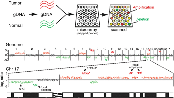

Fig. 3.3
Genomic profiling by array CGH. Above, schematic depiction of array-based comparative genomic hybridization (aCGH). Genomic DNA isolated from tumor and normal reference is labeled with two different fluors (here pseudocolored red and green), then co-hybridized to the array. For each gene on the array, the ratio of red/green fluorescence reflects its relative DNA copy number in the tumor compared to normal reference. Below, tumor/normal log2 ratios (here, for a hypothetical breast cancer sample) are plotted according to reference genome position, shown for the whole genome and for an enlarged view of chromosome 17. Red and green ratios indicate DNA gain and loss, respectively, some corresponding to known cancer genes (e.g., ERBB2, TP53), while other focal amplicons and deletions pinpoint novel cancer genes.
In contrast to expression profiling, analysis of aCGH data emphasizes genome position information. Tumor/normal log fluorescence ratios are first normalized for each array so that the average log ratio is set to zero. As such, CNAs are defined relative to the average copy number for the sample (which may well vary from diploid). Normalized tumor/normal ratios are then mapped onto an ordered representation of the normal genome sequence, where DNA gains and losses are identified as ratio peaks and valleys (Fig. 3.3). Note, this method does not reveal the actual location of CNAs in the cancer genome, where it is known for example that DNA amplification can occur in situ on the chromosome (homogeneously staining regions) or elsewhere in the genome, even extra-chromosomally (double minutes).
Because genomic DNA comprises a more complex mixture of DNA sequences compared to the subset of expressed genes (transcripts), aCGH presents additional technical challenges compared to expression profiling. Further, accurate quantification of very small ratio-fold changes, like single-copy tumor DNA gains and losses in admixtures of normal DNA stromal contamination, is key to localizing and discovering new cancer genes. The sensitivity of detecting low amplitude and focal aberrations is dependent on many factors, including the performance characteristics of the array platform and the density of probe coverage across the genome, with the trend moving towards arrays with 100,000 or more oligonucleotide probes. Measurement accuracy can be improved by averaging ratios across neighboring probes, though at the expense of spatial resolution. Statistical algorithms (and corresponding software tools) are available to call gains and losses in aCGH data [64, 65] and to identify loci recurrently gained or lost across tumor samples [66, 67]. Such recurrently aberrant loci are more likely to harbor cancer genes whose altered copy number and expression provides selective growth advantage, rather than represent secondary inconsequential alterations resulting from genomic instability.
While the above discussion centered on somatic CNAs, germ line DNA copy number variants (CNVs) are increasingly recognized as a source of hereditable variation [68]. CGH arrays can be used to identify CNVs, some of which might be associated with increased cancer risk, or represent preferred sites of tumor genome rearrangement. In defining somatic CNAs, the use of normal reference DNA matched from the same individual can assist in discriminating between somatic CNAs and germ line CNVs.
3.5.2 Single Nucleotide Polymorphism (SNP) Arrays
DNA sequence changes are a major source of heritable variation, and measuring DNA sequence variation was a major motivation for developing DNA microarray technology. Single nucleotide polymorphisms (SNPs) are present on average every 300 bp in the human genome [69], and several million SNPs have been characterized [70]. Affymetrix SNP arrays [71] comprise oligonucleotide probes spanning tens of thousands of SNPs, with separate probes matching the major (i.e., more frequent) and minor SNP alleles (A and B), and can be used to type alleles by DNA hybridization. In brief, target genomic DNA is digested with a restriction endonuclease, and then PCR amplified (using ligated universal adapters) and biotin-labeled for hybridization. Array probes are designed to detect SNPs predicted to reside on restriction fragments within the preferred PCR size range (~0.25–2 kb), and the PCR step serves to reduce target complexity, thereby improving assay performance. SNP genotypes (AA, AB, or BB) are called based on relative hybridization intensities for allele-specific probes. Illumina BeadChip arrays provide a distinct approach with comparable performance for SNP genotyping [72].
SNP arrays can be used to genotype SNPs for whole-genome scan genetic linkage and association studies [73], for example to discover loci conferring cancer risk [74]. SNP arrays can also be used to identify somatic DNA aberrations in tumors, including both CNAs, by scoring hybridization intensity, and LOH, by scoring allelic loss (at informative heterozygous loci) along chromosome segments [75, 76]. Because LOH can result in loss of genetic information in the absence of deletion, SNP arrays can provide additional information useful for mapping tumor suppressors.
3.5.3 Genomic Profiling—Applications
The major application of genomic profiling by CGH (or SNP) arrays has been the discovery of new cancer genes. CGH on microarrays affords orders of magnitude higher mapping resolution compared to prior cytogenetic methods, and has revealed hitherto unappreciated complexities of CNAs in cancer genomes [60, 77]. In various tumor types, recurrent CNAs have been identified that do not contain known cancer genes, and therefore presumably pinpoint new cancer genes. Functionally validated cancer genes discovered by genomic profiling include PPM1D (at 17q23.2), a negative regulator of TP53 amplified in breast cancer [78], and MITF (3p14.1), a master transcriptional regulator of melanocytes amplified in melanomas [79]. Indeed, the discovery of MITF amplification suggested the concept of lineage-dependency oncogenes, where the aberrant expression of genes with key roles in normal cell lineage proliferation or survival is required for tumor cell survival in certain genetic contexts [80]. Another such example is NKX2-1 (TITF1), a transcriptional regulator of normal lung development recently found amplified by genomic profiling of lung cancers [81–83].
Stay updated, free articles. Join our Telegram channel

Full access? Get Clinical Tree


