Cancer Epidemiology

Epidemiology is the study of distribution and determinants of disease and disease outcomes in human populations. The primary research question for epidemiologists is why individuals, or different populations, have different risks of disease or disease outcomes. Epidemiology is broadly focused, examining a full spectrum of disease determinants. These encompass biological, environmental (including lifestyle), social, and economic factors. Consequently, concepts and methods from other disciplines, such as biological sciences and sociology, are critical to the design, conduct, and analysis of epidemiological studies. Important contributions are also made from the field of statistics. Epidemiology provides a critical link between clinical or laboratory results and observed health effects in populations. An observational approach is often the only way to examine risk between disease and a specific risk factor because, for example, it is unethical to assign individuals to an arm of a randomized trial that exposes them to a suspected carcinogen.

3.1.2 General Approach

Epidemiology is often dichotomized into 2 disciplines: descriptive and analytical. Descriptive epidemiology primarily describes rates of disease in populations, either over time or across geographic areas. Analytic epidemiology focuses on individuals in the population, comparing diseased to nondiseased members to determine what factors increase risk for disease. Measures commonly used in descriptive epidemiology are described in Section 3.2. Measures used in analytical epidemiology are described in Section 3.3.

3.1.3 Role of Epidemiology in Translational Medicine

Whereas in vitro and in vivo studies using cell lines and animal models can control for a multitude of experimental conditions, this is difficult in studies in humans. Ethical and feasibility considerations prevent deliberate repeated exposures of known carcinogens to human subjects and randomization of human groups to receive either inferior therapies or environmental exposures. Although some experiments in humans may utilize intermediate subclinical end points that are reversible following brief exposure to a potential carcinogen, these intermediate end points are often not a replacement for the clinical outcome of interest. An example of this type of intermediate end point is the measurement of carcinogen-adduct formation in humans after a single exposure to a putative carcinogen. Such results may support the role of such a carcinogen, but do not provide evidence of increased rates of cancer in individuals or groups of individuals exposed to the putative carcinogen. In general, the process of translating basic science discoveries into the clinical setting requires studies of humans, their biological specimens, and associated clinical data. Such studies require consideration of many factors that can affect the development of disease or its outcome. This is particularly important in the era of microarrays and gene sequencing, where a large number of biological parameters must be considered alongside clinical and epidemiological factors, all of which could affect risk of the disease or outcome of interest.

In the face of such analyses epidemiological principles become important. The majority of epidemiological studies involve observational data (whether aggregate or individual data) where, by definition, the investigator can only observe the characteristics of the population of interest, and cannot intervene to standardize exposures and other factors (such as confounders, see Sec. 3.2.4) that may affect the outcomes of interest. Thus, a key feature of epidemiology has been the development of methodological designs and tools to account for such confounders. These same tools can be adapted for analyses of biological parameters.

Epidemiological studies can serve not only to validate biological principles and translate findings into the clinical setting, but their findings can lead to new avenues of basic research. For example, long before the existence of an activating epidermal growth factor receptor (EGFR) mutation was found to drive certain lung tumors that are highly sensitive to small molecular inhibitors (see Chap. 7, Sec. 7.5.3) there were clinical and epidemiological clues to the existence of a biologically distinct subset of such patients. Patients with tumors that were highly sensitive to EGFR inhibitor drugs were more likely to be lifetime never-smokers, of Asian descent, who had developed the histological subtype of adenocarcinomas, and were (more often) female (Coate et al, 2009). In another example, there has been a dramatic increase since 2000 in the incidence of oropharyngeal cancers, an anatomic subset of head and neck squamous cancers. The patients in this subset were more likely to be younger, lifetime never-smokers, have lower rates of alcohol use, and be of higher socioeconomic status, when compared to the traditional head and neck cancer patient. As time went on, these oropharyngeal cancers were found to be associated with human papillomavirus infection (see Chap. 6, Sec. 6.2.3; Chung and Gillison, 2009). The relationship between alcohol and head and neck cancer is discussed in more detail in Section 3.5.3.

3.2 DESCRIPTIVE EPIDEMIOLOGY

3.2.1 Incidence, Mortality, Case Fatality, and Age-Standardized Incidence Rates

An incidence rate refers to the number of new cases of a disease observed in a defined population in a specific time period divided by the population size, whereas mortality rate refers to the number of deaths caused by the disease during a specific time period divided by the population size. A more precise definition would use the term person time instead of population size. For example, in a town with a population of 40,000 the number of new cases of cancer in a year can be thought of as being divided by 40,000 person-years, 1 year of person time per individual, with the assumption that everyone lived there for the entire year (births, deaths, and migration during the year are ignored). Similarly, the mortality rate would be calculated as the number of deaths from cancer in a year divided by 40,000 person-years.

A direct calculation of incidence rate, as determined in the above example, is termed the crude incidence rate, because the calculation is performed without consideration of other important factors that may differ across different populations. A major factor in the comparison of different populations is the difference in age-distribution across the different populations. Both cancer incidence and mortality generally increase markedly with age, and comparisons of populations with different age distributions using crude rates can therefore be misleading. One can statistically eliminate or reduce the effect of age in the calculation of the incidence of cancer (or of any other disease), and allow comparison of cancer incidence in communities or geographical regions with different age distributions or in the same community with changing age distribution. The procedure requires adjusting (or standardizing) rates so they are representative of the age distribution of some reference population. The reference populations can be chosen arbitrarily to have any age distribution, but typically, the standard population is often conveniently and practically chosen to be the age distribution at a particular census date of the relevant country (eg, U.S. year 2000 census). Different age-standardized rates can then be compared to each other, if they are adjusted to the same reference standard. Figures 3–1 and 3–2 show examples of age-standardized cancer incidence.

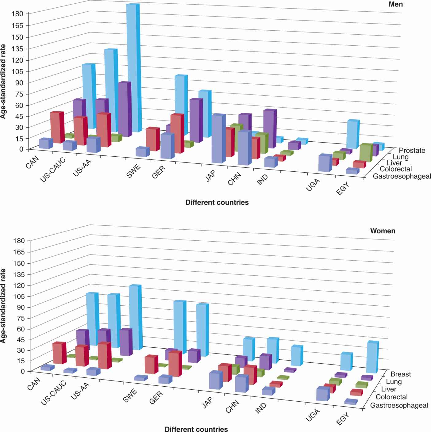
FIGURE 3–1 Comparison of age-standardized incidence rate of selected cancers in selected countries, by sex, per 100,000 person-years. X-axis is divided into different continents: CAN, Canada; US-CAUC, United States caucasians; US-AA, United States African American; SWE, Sweden; GER, Germany; JAP, Japan; CHN, China (Shanghai Registry); IND, India; UGA, Uganda; EGY, Egypt (Gharbiah Registry). Z-axis: dark blue, gastroesophageal cancer; red, colorectal cancer; green, liver cancer; purple, lung cancer; light blue, prostate cancer (men), breast cancer (women).

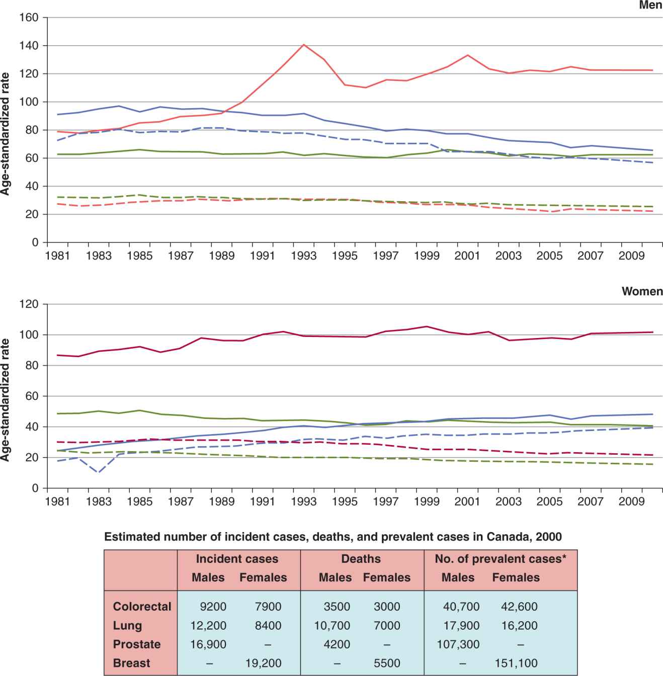
FIGURE 3–2 Age-standardized incidence and mortality rates across 20 years, and incidence, death and prevalence estimates for the year 2000, Canada. (Top) Age-standardized incidence (solid lines) and mortality (dashed lines) rates for lung (blue), colorectal (green), breast (dark red), and prostate cancer (bright red) in Canada, per 100,000 person years for years 1981 to 2010. (Bottom Table) For the year 2000, incident cases, cancer-specific deaths, and number of prevalent cases. *One-year prevalence, 2000. (Data from Canadian Cancer Statistics, 2010.)

The age-standardized rate is commonly presented in publications as it accounts for differences in age between populations or changes in age within populations over time. However, such adjusted rates should be viewed as relative indices rather than actual measures of occurrence. Rates can also be compared within age groups.

The age-specific incidence rate is defined as the incidence of disease in a specific age group; typically, 5-year age groups (0 to 4, 5 to 9, 10 to 14, etc) are used. This method is informative about the disease pattern over the life course, but a valid comparison across populations can only be made within age groups.

The case fatality rate is the number of deaths caused by a specific disease in a defined population divided by the number of individuals who have been diagnosed with that particular disease, in a fixed time interval. Only deaths among those diagnosed in the time interval are included in the numerator. An example of a case fatality rate is found with breast cancer, which in the Western world is around 25 individuals per 100, or 25%. This means that within a given year, of every 100 individuals carrying a diagnosis of breast cancer in a population, 25 individuals in the same population will have died of breast cancer. Contrast this result with pancreatic cancer, where the case fatality rate is more than 95%; that is, of 100 individuals carrying a diagnosis of pancreatic cancer, more than 95 patients will have died.

3.2.2 Prevalence

Prevalence is defined as the proportion of a population that has a disease at a specific time point (prevalent cases divided by population size), where prevalent cases include both new cases of disease and the number of previously diagnosed cases who are still alive in a population. Including all cases who are still alive as prevalent cases assumes that no cases can be considered cured. This raises the question of whether long-term survivors of cancer should be included in the prevalence group when calculating prevalence. Given the available data (which may not include treatment information), decisions should be made that ensures the prevalence calculation reasonably reflects the burden of disease in the population. For example, one can define prevalent cases as those diagnosed and still alive at the end of a specified time period (eg, the last 5 years).

Prevalence is a function of both cancer incidence and cancer survivorship (ie, how long the person lives with the disease or disease chronicity). As an example, although lung cancer ranks among the most common cancers in the Western world, its prevalence ranks lower than that of prostate cancer, breast cancer, and colorectal cancer, because lung cancer is such a lethal disease. Both cancer incidence and cancer prevalence are important measures. Cancer incidence reflects how commonly cancer develops in a population, and the impact of preventive measures and health service utilization related to initial diagnosis and treatment. In contrast, cancer prevalence may be important when considering the overall burden of a cancer on a global health system, and longer-term impact on survivors.

Figure 3–2 shows the relationship between incidence, mortality, and prevalence. In lung cancer, the dashed (mortality rate) line approaches the solid (incidence rate) lines, which represents a low survival rate (of approximately 10% to 20%). The low survival rate results in a low prevalence of disease in the population, as a high proportion of lung cancer patients die of their disease, resulting in few long-term survivors. For prostate, breast, and colorectal cancers, the age- standardized incidence rates are substantially higher than their corresponding mortality rates, as a result of high survival rates (all greater than 40%). In the figure, both the age-standardized incidence of prostate cancer and the incidence–mortality gap for prostate cancer in men was similar to the same indicators for breast cancer in women. Because prevalence is a function of incidence and survivorship, one would have expected a similar prevalence of prostate cancer and breast cancer patients in 2000. Yet there was approximately 50% more prevalence in breast cancer patients when compared to prostate cancer patients. The reasons for this finding are (a) women live longer than men, on average, and (b) the median age of diagnosis of breast cancer is lower than that of prostate cancer. Thus, in the year 2000, a breast cancer patient can expect to live longer, on average, than a prostate cancer patient, leading to a greater prevalence of breast cancer patients when compared to prostate cancer patients (see Fig. 3–2). This aspect of survivorship links incidence, mortality, case fatality rates, and survivorship characteristics with prevalence rates.

3.2.3 The Role of Sampling

A major focus of epidemiology is to identify associations that are true for an entire population. Optimally, one would collect exposure and disease status data from every member of that population. If the information collected is accurate, then any associations found would be true.

In the real world, it is not feasible to collect data from the entire population, and a subset of the population is studied. Even the most comprehensive national census data from countries that make completing a census mandatory will have certain individuals refusing to comply (typically the disenfranchised, those not in the country legally, and any groups that are suspicious of government oversight). In many cases, because of cost and feasibility, basic census data are collected from as many individuals as possible, while detailed comprehensive information is collected from a subset of the population. Sampling is therefore a key component of epidemiological analyses. The goal of sampling is to evaluate a subset of the population where the exposure and disease status information is representative of the underlying population. In an ideal setting, the results found in the sample should fully reflect the true associations in the underlying population. When the results are different, bias and measurement errors may explain these discrepancies.

3.2.4 Types of Bias

A study is biased if the results are different than the truth. In epidemiology, bias can be viewed as a distortion of risk estimates from their true values. Bias can be related to the identification of cases, measurement of exposure, improper analysis of results, or systematic errors in data collection and entry. Many different kinds of biases have been described (Sackett, 1979; Szklo and Nieto, 2007). We describe the main types of bias found in observational studies, including confounding, selection, and information bias.

3.2.4.1 Bias Because of Confounding An important bias in observational studies comes from confounding, defined as the distortion of effect of an exposure on risk (of disease or outcome) that arises because of an association with other factors that affect such a risk. Confounding can lead to spurious associations, mask associations that are real, or distort the strength of an association. A variable is considered to be a confounder if it is associated with the potential disease-related factor under investigation (either causally or noncausally) and is causally related to the outcome of interest (either risk of disease or its outcome). An example of a confounder is smoking in lung cancer (Fig. 3–3A). Suppose we are studying the association between tooth loss and lung cancer risk. Tooth loss, a marker of poor hygiene, is strongly associated with heavy smoking. We may therefore find an association between tooth loss and lung cancer solely because both are associated with heavy smoking. In reality, tooth loss does not lead to lung cancer development, but its association with smoking makes it appear that it is related with lung cancer risk, while the true association is between smoking and lung cancer.

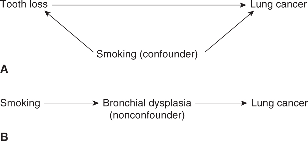
FIGURE 3–3 Confounding in epidemiologic studies. The confounder is related to both the exposure of interest and to either disease or outcome. Example A reflects confounding by smoking. Example B is not an example of confounding because bronchial dysplasia lies in the causal pathway leading to lung cancer.

A variable is not considered to be a confounder if it lies in the same causal pathway as the potential disease-related factor under investigation. For example, bronchial dysplasia is an intermediary in the pathway between smoking and lung cancer, and is thus not a confounder (see Fig. 3–3B).

In summary, there are 3 criteria for a variable to be a confounder:

1. A confounding factor must be a risk factor for the disease;

2. A confounding factor must be associated with the exposure under study in the source population; and

3. A confounding factor should not be an intermediate factor in a causal path between exposure and disease.

Confounding can be dealt with in different ways. Individuals who have a disease (eg, cancer cases) and those without disease (eg, healthy controls) can be matched on potential confounding exposure variables (eg, age and sex are commonly matched in a case-control study) to reduce or eliminate confounding by these variables, or data can be analyzed within specific strata of the confounding variable (eg, analyses stratified by ethnic group). In addition, one can control for confounding using multiple regression analysis, which is discussed in Section 3.3.3.

3.2.4.2 Selection and Information Bias Sometimes the results of analyses of a sample will differ from the true associations in the underlying population. This may be a result of sampling problems, whereby the sample selected does not represent the underlying population. Selection bias refers to systematic differences between those who participated in the study versus those who should be theoretically eligible for the study (including those who do not participate). An example of sampling bias results from recruiting cases from a surgical clinic to represent the entire population of stomach cancer. Because surgeons generally see more early stage patients (ie, those who are operable), the population will be skewed toward earlier stage patients, where as the whole population of patients with stomach cancer is eligible for the study.

Information bias occurs as a consequence of errors in obtaining the needed information, which is often termed misclassification or classification error. Sometimes these misclassifications can lead to results from studies that do not represent the true associations in the underlying population. An example of information bias occurs if lung cancer patients overestimate their exposures to asbestos (compared with healthy controls) while underestimating their own cigarette smoking history (perhaps as a means of reducing their own culpability in developing this disease). The resultant effect is a smaller-than-true risk associated with cumulative smoking, and an exaggerated risk associated with asbestos. This bias particularly affects case-control studies (see Sec. 3.4.3) where cases are recruited after their diagnosis, and is referred to as recall bias. Such a bias would be absent if individuals were asked for their exposure status prior to developing their cancer (as in the case of cohort studies; see Sec. 3.4.2). Another example of information bias may come from evaluating a molecular test. Assume that the molecular test categorizes individuals into 3 levels: A, B, and C. However, because the test is inappropriately calibrated, a number of B test results are misclassified as C results, whereas B results are never misclassified as A results. The resultant error is directional in nature (ie, nonrandom).

Although systematic error such as selection bias and differential misclassification can generate biases in epidemiological studies, random error can also distort the results of epidemiological studies. Random error is the deviation that arises by chance between the observed value (in the sample) and its true value (in the underlying population). The greater the random error, the less precise the result.

Assessment of cancer diagnosis should be reasonably accurate as diagnosis is generally verified with a pathology report. The determination of cause of death can be more problematic if death certificates are used. Assessment of exposure can be particularly problematic, and misclassification of subjects with respect to their exposure can be extensive. Recall of certain past exposures, such as diet, may show considerable random error. Error in the measurement of biomarkers depends not only on the accuracy of the bioassay, but how well a single measurement may reflect long-term levels of the biomarker. The latency period for cancer can be many years and a single measurement of a biomarker during an individual’s lifetime may not effectively represent long-term levels.

Generally, misclassification of a dichotomous (ie, positive or negative) exposure will lead to a bias toward the null (relative risk estimates will indicate a smaller association than actually exists or indicate no association when true association is present), and when the misclassification is extreme the result can go beyond null to the opposite direction. However, misclassification of a multilevel exposure could lead to errors in any direction. Efforts to increase the accuracy of assessment of exposure or use of large samples that can detect the attenuated associations are the only ways to address this problem. We discuss some of the newer strategies in Section 3.7.2. Table 3–1 defines and describes other common examples of selection and information biases.

TABLE 3–1 Types of selection and information biases in epidemiological studies.

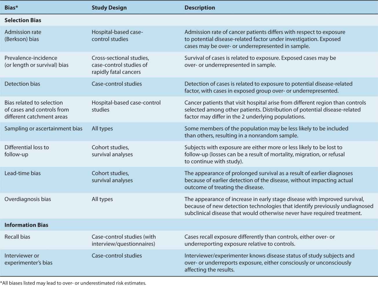
3.2.4.3 Bias in Cancer Screening Two special causes of bias are related to cancer screening. These biases can affect incidence, prevalence, mortality, and survival rates. For example, as Figure 3–2 shows, prostate cancer incidence rates had 2 separate peaks (1993 and 2001). Each peak was related to the clinical adoption of a screening test based on the serum levels of prostate-specific antigen (PSA). The first peak followed initial adoption of the PSA test, while the second peak may be explained by increased PSA testing related to the publicity around a prominent Canadian politician’s prostate cancer diagnosis (Canadian Cancer Society, 2010). New screening techniques may result in individuals with subclinical prostate cancer being diagnosed earlier than traditionally expected. In the absence of the screening, the prostate cancers would be detected at a later date, when the subclinical cancer grows large enough to produce symptoms and be detected using previous methods. At the time of clinical adoption of such screening, survival may be prolonged because there is a true benefit of screening and the cure rate has truly risen. However, 2 potential biases complicate the interpretation of findings. Lead-time bias and overdiagnosis bias may have accounted partly for these peaks.

Lead-time bias refers to the appearance of longer survival after diagnosis that is a result of diagnosis at an earlier time during the course of the disease, and thus a longer time that the patient is known to have the cancer rather than an improved treatment response. The fact that early detection may not necessarily benefit the patient clinically, because the patient may have died at the same time with or without screening, is an important consideration when evaluating cancer screening programs. In the context of screening, length time bias occurs when screened subjects with better prognosis are detected by a screening program. This can result from more rapidly growing (and more lethal) cancers being diagnosed outside of the screening program, thus leading to an impression of better survival among screened subjects (see Chap. 22, Sec. 22.3.3).

Screening can also lead to overdiagnosis bias. PSA screening may lead to the detection of subclinical cases of prostate cancer that would never have become clinically diagnosed in individuals who would have eventually died from an unrelated cause. Nonetheless, overdiagnosis results in increase in cancer incidence, apparent prolonged survival after diagnosis (and, therefore, apparent decrease in case fatality rates), and greater prevalence of the disease, all as a result of the new detection of previously subclinical disease that has no real clinical relevance.

3.2.5 Geographic Variation

Geographic variations in cancer incidence can be a result of differences in prevalence of the underlying causes including environmental and ethnic (ie, genetic) differences, or to differences in diagnostic criteria. In addition, geographic comparison can be complicated by differences in screening, which, by detecting occult disease, usually has a much larger effect on the incidence of disease than on mortality (see Chap. 22, Sec. 22.3.3). Figure 3–1 shows the age-standardized incidence rate for selected cancer sites and countries. Some large variations can be observed across countries, and there may also be large variations within countries: for example, the rate of esophageal cancer varies by 10-fold within Iran (Saidi et al, 2000). In another example, shown in Figure 3–4, there is substantial geographic variation in incidence rates of liver cancer (Ferlay et al, 2010). The highest incidence rates are observed in sub-Sahara Africa and Asian countries such as China (~25 per 100,000 person years), Thailand (~30 per 100,000 person years), and Taiwan (~35 per 100,000 person years), whereas lower rates are observed in Europe and North America. This variation is partially accounted for by the prevalence of chronic infection with hepatitis B and C virus (HBV and HCV), which are causally associated with 80% to 95% of liver (hepatocellular) cancer (Maupas and Melnick, 1981). Similarly, the variation of cervical cancer can be partially accounted for by the prevalence of human papilloma virus (HPV), as we now know that cervical cancer is associated strongly with a few of the oncogenic genotypes of HPV (Munoz et al, 2003). Infection and cancer is described in more detail in Section 3.5.1 (see Chap. 6, Sec. 6.2.3).

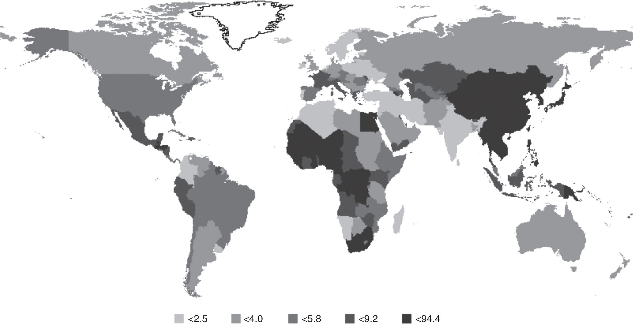
FIGURE 3–4 Global variation in incidence of liver cancer. Annual age-standardized incidence rate, per 100,000 person years, across different countries of liver cancer. (From Ferlay et al, 2010 with permission.)

3.2.6 Time Trends

Figure 3–2 shows the age-standardized incidence rate (ASIR) of the most common cancer sites in Canada for males and females in the last 20 years. Lung cancer incidence rates in men have been decreasing steadily since mid-1980s from approximately 90 to 65 per 100,000 person years in 2010, whereas the lung cancer incidence rate in women continues to rise from approximately 25 per 100,000 to 48 per 100,000 person years in 2010 (Canadian Cancer Society, 2010). The long-term projection suggests that this trend is beginning to level off. This pattern corresponds to the patterns of tobacco consumption in men and women with a lag time of approximately 20 years. In contrast, colorectal cancer rates have remained relatively stable over the same period. Breast cancer incidence has slightly increased during this period. Changes over time for prostate cancer incidence rates have already been discussed in Section 3.2.4.3.

Worldwide, the incidence rate of stomach cancer in men has been decreasing in the last 30 to 40 years. Regardless of the steady decline, stomach cancer was still the fourth most common incident cancer worldwide in 2008 following cancer of lung, breast, and colorectum (Ferlay et al, 2010). In contrast, the incidence of thyroid cancer is increasing most rapidly among all cancers and it has doubled in women in the last 10 years, in both Europe and parts of the United States (Lundgren et al, 2003; Davies and Welch, 2006). The increase in incidence of thyroid cancer is mainly observed for papillary thyroid cancer and it may be a result of the change in the morphological recognition of this tumor (Lundgren et al, 2003). More frequent use of medical imaging may also contribute to the increased detection of early stage, asymptomatic cancers. The mortality of thyroid cancer did not show any increase during the same period of time.

In addition to adult cancers, recent publications based on the Automated Cancer Information System focused on childhood cancer have provided detailed statistics of major childhood cancer in Europe between 1978 and 1997 (Kaatsch et al, 2006). This analysis, based on 33 cancer registries in 15 European countries, showed an increased rate of childhood cancer in all regions for the majority of tumor types, including soft-tissue sarcoma (annual rate of increase 1.8%), brain tumors, tumors of the sympathetic nervous system, germ cell tumors, and leukemias (annual rate of increase 0.6%). Diagnostic methods can only partially explain the upward trend, and factors such as changing lifestyle and environmental exposures may be important.

3.3 ANALYTICAL EPIDEMIOLOGY

3.3.1 Basic Comparative Approaches: Relative Risk, Odds Ratio

The relative risk measures the risk in a group exposed to a potential disease-related factor and compares it to the risk in a group that is not exposed (or has lower exposure) to the factor. The risk itself may be to developing a specific cancer, or to a specific cancer outcome. In a population-based study of cancer risk, individuals who develop cancer and those who do not are classified into exposed and nonexposed groups according to their baseline measures, which are taken well before any individuals have developed cancer. In a population study of cancer outcome, individuals who develop a specific outcome (eg, response to therapy or drug toxicity) and those who do not are classified into exposed and nonexposed groups. In either example, the relative risk can then be calculated by dividing the risk of disease (or outcome) in the exposed group by the risk of disease (or outcome) in the unexposed group, as shown in Figure 3–5. Another related measure of relative risk is the rate ratio. It can be calculated when disease (eg, incidence) rates (Sec. 3.2.1) are available, by dividing the rate of a disease in a group exposed to a specific factor by the rate in a group that is unexposed or has lower exposure to the same factor. The rate ratio is useful in comparing populations in defined geographic areas with different exposures (eg, cigarette smoking or industrial pollution).

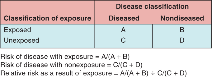
FIGURE 3–5 Calculation of relative risk of disease. (The letters A, B, C, and D refer to number of subjects in each group.)

A relative risk of 1 (or more precisely a relative risk not statistically different than 1) indicates that there is no detectable increased risk of disease (or outcome) in the exposed group. A relative risk greater than 1 indicates risk is increased among the exposed, and a relative risk of less than 1 indicates lower risk in exposed verses unexposed groups. The farther away the value is from 1 (either very large numbers or very small numbers), the stronger the association.

Within either the entire population or a representative subset, the relative risk can be directly calculated because the size of both the exposed and unexposed groups from which cancer cases arose is known. In contrast, if a study selects cases from a population and then compares them to a selected set of controls, the size of the underlying exposed and unexposed groups in the population, and therefore the relative risk, cannot be directly calculated. Instead, the odds ratio must be calculated as outlined in Figure 3–6.

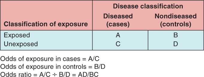
FIGURE 3–6 Calculation of the odds ratio. (The letters A, B, C, and D refer to number of subjects in each group.)

The odds ratio is generally presented as an approximate measure of relative risk. This approximation is valid if the prevalence of the disease is relatively low in the population, typically less than 10%. Although prevalence of all cancers together is relatively high in most Western populations, the prevalence of each individual cancer is quite low. This approximation can be demonstrated by starting with Equation 3.1 for the calculation of relative risk. If the disease is rare, then only a small change to the resulting estimate will be seen if both A (subjects with exposure and disease) and C (subjects with no exposure and disease) are removed from the denominator of the first and second parts of the equation (Eq. 3.2). The resulting equation can be rearranged so that it is identical to the equation for the odds ratio (Eq. 3.3).

The relative risk and odds ratio show strength of association, and are as applicable to analyses of relationships of biomarkers with disease as to clinicoepidemiological relationships.

3.3.2 Probability, Distributions, and Tests of Association

Let us assume that in the South Pacific there are exactly 1000 adult islanders (age 18 years and older) living on a remote atoll (Island A). On this island, 400 individuals have high blood pressure. If we are allowed to check for high blood pressure in 100 islanders (ie, sampling the population), we may obtain 40 with hypertension, but we may by chance, also obtain 39, 38, 37, or 41, 42, 43 individuals with high blood pressure, but it would be highly unlikely to obtain either no individuals with high blood pressure or all 100 individuals. If we repeated the experiment a million times, each time sampling 100 individuals randomly, the most frequent result will be 40 individuals with high blood pressure, with other results farther away from 40 (in either direction) being less frequent. These results, if plotted, will form a shape similar to a normal distribution or probability curve (note: with two possible outcomes, hypertensive or not hypertensive, the distribution is in fact binomial but approximately equal to the normal distribution given the large number of data, thus leading to a bell-shaped [normal] curve; see Fig. 3–7). If we obtain a value from a sample that falls outside a certain range of values, then we might conclude it is highly unlikely that the value comes from a population similar to the Island A population. This range is conventionally chosen to be the 95% confidence interval, in which case the top and bottom 2.5% of values are considered to be too different to be likely to have come from the Island A population. Under different circumstances and depending on the experimental design of each study, different distributions or curves may be more appropriate, as would different ranges of confidence intervals.

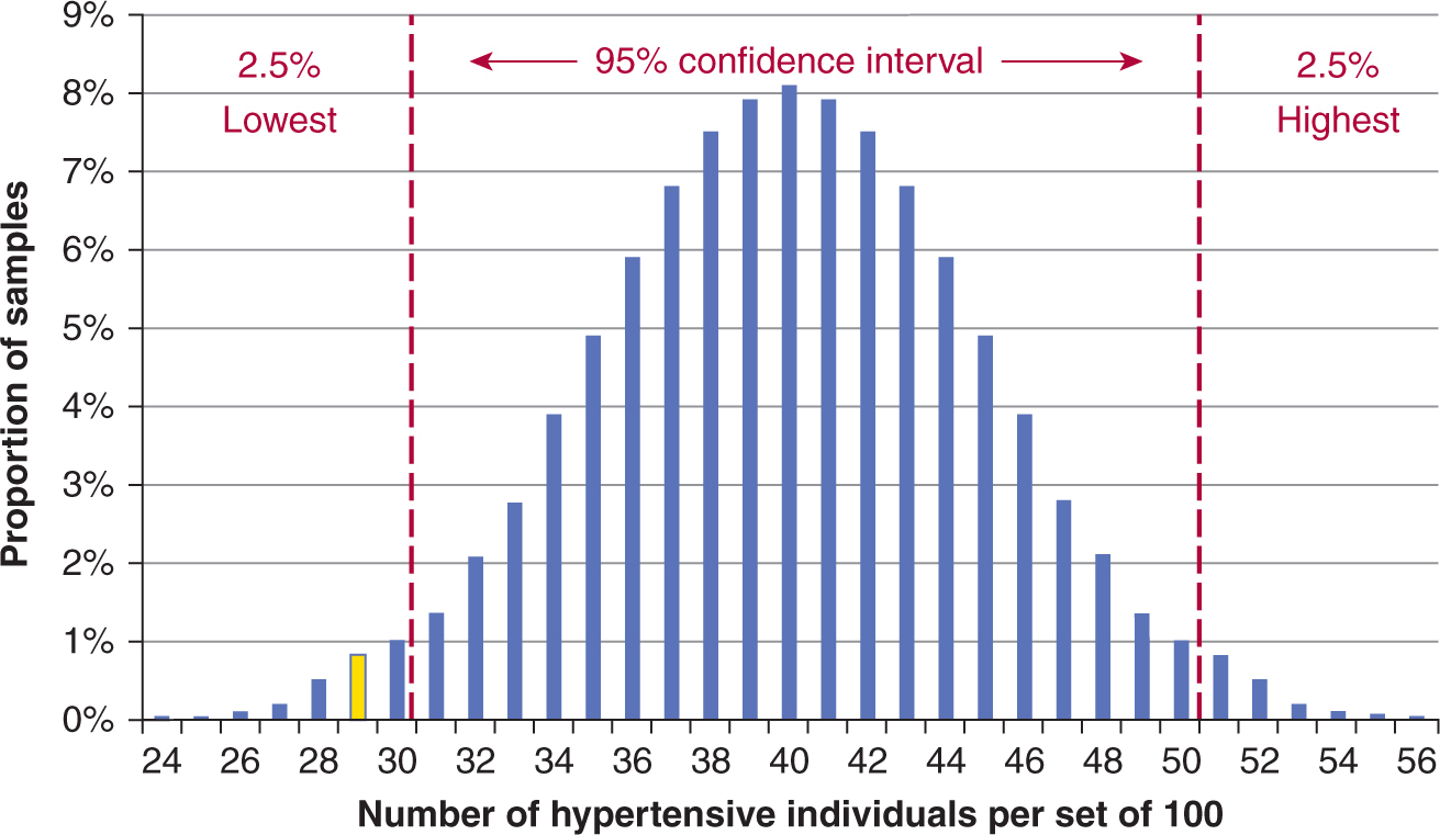
FIGURE 3–7 Normal distribution approximation of binomial distribution for a 100-patient sample for a 40% proportion. Assume that an underlying adult population has a 40% prevalence of hypertension. Researchers repeatedly and randomly sampled 100 individuals from this population (Island A), and reported the prevalence of hypertension in each sample. The X-axis shows the number of hypertensive individuals in each set of 100. The Y-axis shows the proportion of samples with that number of hypertensive individuals. The 95% confidence interval (within which 95% of these samples fall, around the median of 40) is shown in between the red dotted lines. The results in the yellow bar represent the proportion of samples that had 29 hypertensive patients (Island B).

If on a sister island (Island B) with 1000 people, we sample 100 individuals once and find that 29 of them have hypertension (Fig. 3–7, yellow bar), are the individuals on Island B similar to Island A? From Figure 3–7, the chance of this happening if the population of the 2 sets of islanders have the same risk of hypertension is found to be outside of the 95% confidence interval. We conclude that Island B’s population has a different risk of hypertension than Island A’s population.

A chi-squared (χ²) and t-test are different tests for association. Each is based on an underlying distribution and compares the result of one group with that of another. The tests are considered significant when the 2 groups are thought to be too different from each other for the variable of interest to have come from the same underlying population. Chi-squared tests evaluate variables that are discrete categorical values (ie, ex-smoker, current smoker, never smoker; or male, female), whereas t-tests evaluate continuous variables (eg, hormone levels, age).

3.3.3 Regression Approaches

Sometimes, one wants to compare more than one variable or factor (also known as a predictor or independent variable) with disease risk or outcome (the dependent variable) simultaneously. Chi-squared and t-tests can only evaluate 1 variable at a time. Regression techniques are statistical methods to examine the association of multiple potential disease-related factors with disease or disease outcome. Multivariate regression analysis also permits simultaneous inclusion of many covariates (ie, factors) that are essential in controlling for confounding. In essence, this allows for consideration (and adjustment) of multiple factors in the same analysis. Including multiple variables in the same model is the equivalent of asking what the true association of the factor of interest is when many other predictor variables are simultaneously considered together. In biomarker and biospecimen analyses, such factors of interest can involve protein levels, immunohistochemical staining patterns, serological levels, germline variation, somatic mutations, and epigenetic markers, while clinicoepidemiological factors may include, age, gender, patient comorbidities and general state of health, tumor grade and histological subtype, disease stage at diagnosis, and treatment.

Regression models generally follow a common pattern. Equation 3.4 represents a univariate analysis where the x represents the value of the independent (predictor) variable, while the y represents the dependent (outcome) variable. β₀ is a nominal constant, while β₁ represents the association between x and y in the model, and its value is a constant that is generated as part of the regression analysis. The more the value of β₁ deviates from 0 (whether a large positive or large negative value), the stronger is the magnitude of association between x and y.

In Equation 3.5, a single model now incorporates multiple (n) independent variables altogether, as predictors of the outcome, y. This type of model is useful if all n variables are being evaluated as predictors of outcome, y. At other times, one is only interested in the association between y and a single predictor variable, x₁, while the other variables x₂ … x, represent potential confounders. Data for each study participant (ie, values for x₁ through x_n and for y) are placed into the regression analysis, and values for β₀ through β_n are generated as part of the regression model.

Table 3–2 describes the various formats in which to incorporate the independent predictors, x_n, into a regression model. Table 3–3 summarizes the format of the outcome variable, y, which determines the type of regression.

TABLE 3–2 Different formats for the independent variable, x_n.

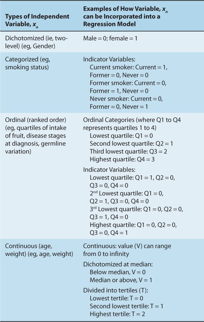
TABLE 3–3 The relationship between type of outcome variable and regression model.

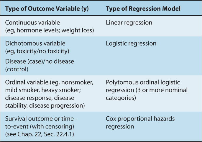
All regression analyses must make assumptions about the nature of their underlying variables x and y. For instance, linear regression analyses assume that a continuous, independent x_n variable will have a linear relationship with the y outcome variable. If this is not true, then the x variable may need to be transformed to a format where a linear relationship between x_n and y exists; these may include taking the square root or taking the logarithmic function of x. In another example, the association between average adult weight and cancer risk may be the result of a threshold effect, in which case, dichotomizing weight at the threshold (rather than treating the variable as a continuous variable) would be more appropriate. In the case of a Cox proportional hazard model, the assumption is that the ratio of hazards (defined as the rate of dying in a short period of time) between the comparator arms remain constant. Many survival curves violate this assumption, most obviously when they cross each other. It is therefore critical that assumptions behind each of these models are checked, and any deviations from these assumptions lead to disclosure and use of alternative methods of analyses (see Chap. 22, Sec. 22.4.1).

A useful property of the logistic regression function is that the β estimates generated in the model are mathematically related to an odds ratio. This relationship is as follows:

3.3.4 Interaction

The term interaction has been used in the context of statistical, biological, and public health concepts. In general, interaction refers to 2 or more factors modifying the effect of one another with respect to outcome. Epidemiologists often refer to this as effect modification. An interaction may arise when considering the relationship among multiple variables, and describes a situation in which the simultaneous influence of 2 variables on a third is synergistic or antagonistic. A classic example is the interaction between smoking and asbestos exposure. Each factor individually increases lung cancer risk, but exposure to asbestos increases the cancer risk in smokers much more than simply adding the 2 risks together.

In cancer, interaction analyses often focus on gene–environment interactions, where the goal has been to identify environmental factors that, in the presence of the right combination of genetic or host factors, substantially modify (typically increase) the risk of developing certain cancers. In the realm of pharmacogenetics and biomarker research, interaction analyses are increasingly important (see Sec. 3.7.1).

Interaction should not be confused with confounding. A confounder has a stable effect on the relationship of the exposure-to-risk and disease-to-outcome variables; proper analysis will “correct” such a confounder effect and produce an accurate estimate of risk for a potential disease-related factor. In an interaction, the risk estimate for the factor changes with different levels of the variable it interacts with, as illustrated in Figure 3–8. Interaction can be explored using regression techniques.

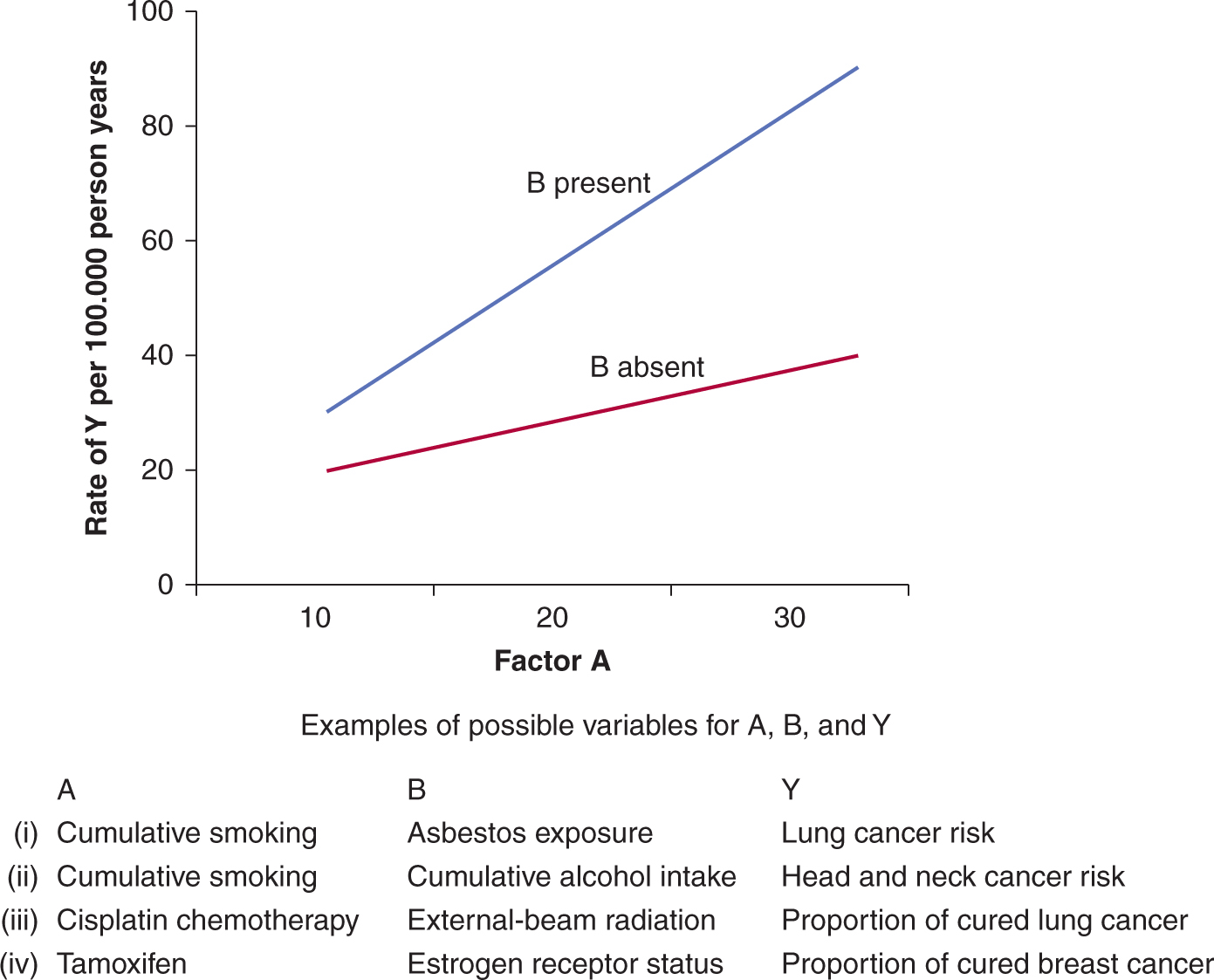
FIGURE 3–8 Interaction between two independent predictors of disease or outcome. In the example, an increase from 10 to 30 units for the factor of interest, A, results in the disease rate increasing from 20 per 1000 to 40 per 1000 when factor B is absent. In the presence of factor B the same increase in factor A results in a much greater increase in disease rate: from 30 per 1000 to 90 per 1000. Factor A interacts with factor B as factor A has a stronger effect on disease rates in the presence of factor B. Note that the examples in the table are not associated with the values given in the graph, which is presented for illustrative purposes.

3.4 ANALYTICAL STUDY DESIGNS

3.4.1 Ecological Design

Ecological studies focus on groups of individuals (or populations) as the unit of observation. These groups may include people living in a defined geographic area, or people from different schools or workplaces. The outcome in these studies is generally the incidence rate (of cancer). For example, an ecological study may look at the association between use of alcohol and incidence of liver cancer in different countries. Measures of exposure to potential disease-related factors are based on aggregate data and can be classified into 3 subgroups:

1. Aggregate measures—characteristics of a group summarized as a mean or median of some putative exposure or the proportion exposed for the group (eg, median or mean income, proportion of smokers).

2. Environmental measures—physical characteristics of the defined area of interest (eg, measures of air pollution).

3. Global measures—characteristics of groups or locations for which there is no analog at the individual level (eg, laws or regulations that reduce exposure to secondhand smoke).

Relative to other study designs, ecological studies are generally inexpensive as data are often readily available. The availability of data can often permit comparisons where exposure differs markedly across populations, such as data representing intake of some foods or nutrients across countries, which may be critical in finding associations.

The most important bias related to ecological studies is known as the ecological fallacy, where associations between aggregate measures of exposure and disease may not represent associations at the individual level. Ecological studies generally assume that all members of a group exhibit characteristics of the group as a whole. When this assumption does not hold, the association for the ecological exposure measure will be flawed and can even be in the opposite direction than that of the individual measure. A commonly cited example is an ecological study that identified suicide rates to be positively correlated with the proportion of Protestants in Prussian communities. An obvious interpretation of this is that Protestants were more likely to commit suicide than other groups in these communities. However, because of the study design, it cannot be concluded that a greater proportion of Protestants were committing suicide. An alternative explanation is that differences in suicide rates between communities might be explained by other groups, such as Catholics, having a higher suicide rate in protestant communities, perhaps because of a feeling of social isolation (Szklo and Nieto, 2007). An ecological design does not allow one to confidently distinguish between these 2 opposing explanations because individual level measures (in this example, information on faith and cause of death for each of the study subjects) are not available.

3.4.2 Cohort Design

A cohort study follows a group of people over time comparing those exposed to a factor that may influence risk or outcome of disease to those not exposed to the factor. Individuals typically enter into a cohort because they meet clear-cut criteria using a defined sampling protocol. Cohorts can be prospective (also called concurrent) or retrospective (nonconcurrent or historical). In a prospective cohort, individual study subjects are recruited at a specific point or range in time. Measurements of potential disease-related factors (baseline measures) are made as individuals are recruited into the cohort, and study subjects are then followed over time with further measurements possible. Because exposed and nonexposed individuals within the study are followed over time, relative risk can be calculated directly (see Sec. 3.3.1 and Fig. 3–5). A retrospective cohort makes use of existing databases for information about disease (usually identifying incident cases or deaths) and the disease-related factor of interest. In specific circumstances, biological samples are also available for translational experiments from these retrospective cohorts, either because they were collected as part of a parallel biobanking process, or because such samples were stored long-term following original diagnostic biopsies. The quality of preservation, the quantity of usable material, and the completeness of collection across the entire cohort should be assessed critically, as should the quality of retrospectively collected clinical and epidemiological information.

Although a typical epidemiological cohort study begins with a healthy population (where risk of disease is the outcome being assessed), a growing number of observational cohorts follow individuals with disease (such as cancer), where the outcomes being assessed are treatment-related responses or toxicity, rates of disease relapse and progression, course of disease over time, and/or overall survival. Sometimes, these disease-specific cohorts are labeled case series. Case series may involve carefully collected sets of patients, but they may also consist of a convenient, haphazardly collected set of available cases. Use of the term cohort implies a well-defined set of patients adhering to specific entry criteria, such as stage-specific, or geographic-specific sets of individuals.

Prospective cohorts have the advantage of allowing investigators to control subject selection, ascertainment of events, and follow-up, and to determine baseline measurements. In most modern large-scale cohort studies, subjects are chosen according to some defining criteria, such as occupation (eg, nurses in the Nurse Health Study) or residing in a particular area (eg, the Ontario Health Study). Generally, incidence of disease is the outcome of interest. Often, multiple diseases (including a variety of cancers and noncancer outcomes) are investigated in 1 study, to maximize its efficiency and cost-effectiveness. Assessments may involve interviews or mailed questionnaires or measures made at a clinic such as height and weight. Biological samples may be taken and stored for later assessment of molecular and genetic biomarkers. Similar to retrospective cohort studies, it is important to assure the quality of such biomaterials. In analyses of disease risk, the advantage of prospective cohort studies over other observational approaches is that exposure to a disease-related factor is measured prior to development of disease; it is this property that makes cohort studies so important in translational science. Assessing the exposure after development of disease can lead to bias. For example, biomarker levels in blood could be influenced by the presence of disease; thus, obtaining specimens well before diagnosis of cancer is important.

Ascertainment of outcome is critical in a cohort study. When the outcome is the development of cancer, a pathology report from a cancer registry is often used to identify the case and confirm the diagnosis. An accurate date of diagnosis is required so that prevalent cases are not counted, and is essential when one of the outcomes is survivorship after diagnosis. When the outcome of interest is response to treatment, toxicity, recurrence, and/or survival, careful standardization for measuring each outcome must take place, usually with systematic repeated evaluations (eg, standardizing a follow-up schedule). Many subjects can be lost to follow-up despite extensive efforts to track them. Losing subjects to follow-up can introduce bias if these losses are differential with respect to either the potential disease-related factor or the outcome of interest. Linkage to cancer registries and mortality databases can permit tracking of individuals so that disease occurrence and vital status can be ascertained even if subjects are lost to routine follow-up. Although overall survival requires a hard outcome measure (alive or dead), loss to follow-up and missing outcome may still require clinical interpretation, whereas other outcomes, such as disease-free survival and cancer-specific mortality may be subject to error or bias.

Prospective cohort studies designed to evaluate risk of disease are very expensive. For a disease such as cancer, many individuals will have to be recruited to ensure that a sufficient number of incident cases will occur for meaningful analyses. Also because cancer has a long latency period, researchers may have to wait for many years after recruitment before sufficient numbers of cases are available for analysis.

Cohort studies of outcomes after cancer diagnosis are also expensive, as a consequence of the costs of performing accurate and careful patient follow-up. In addition, heterogeneity in treatment and patient management is a substantial source of confounding in such studies. Thus, unlike cohort studies of disease risk, typically it is easier to analyze and interpret single-institution studies or studies involving a small number of institutions that follow similar treatment plans, compared to those studies in which treatments are heterogeneous. Yet single-institution studies can suffer because of inclusion of a highly selected subset of patients, limiting generalizability. In contrast, the analysis of cancer registry data for a geographic region, which represents an analysis of what is expected in the real world, may suffer from wide variability in patient management (eg, therapy, monitoring, and follow-up). In many ways, the single-institution observational study may mirror the clinical trial (rigorous entry criteria, uniform therapy, well-defined follow-up), whereas the registry and cohort data may mirror health outcomes research (real world analysis; see Chap. 22, Sec. 22.9).

3.4.3 Case-Control Design

In contrast to a cohort study where incidence of disease is compared in differently exposed groups, case-control studies recruit newly diagnosed cases and compare these to controls with respect to their exposure to a potential disease-related factor. The recruitment of incident cases means that there is no need to wait for disease to occur. This greatly reduces costs relative to cohort studies, particularly for rare diseases, because there is no need to recruit large number of subjects and wait for some to develop disease. In studies of disease outcome, a case-control study typically compares patients with certain outcomes (eg, cancer-free patients; patients without treatment toxicities) to patients with alternative outcomes (eg, patients who have relapsed from disease; patients with significant toxicities from a specific treatment). Relative risk cannot be calculated directly within a case-control analysis, but is estimated using the odds ratio (Sec. 3.3.1 and Fig. 3–6).

Various sampling strategies are employed for case-control studies. In hospital-based studies, patients diagnosed with the disease of interest are recruited, either as cases for an analysis of cancer risk, or as the basis of a nested case-control study of disease outcome (see below). Controls for analyses of cancer risk are obtained from groups of patients whose reason for attendance at an outpatient clinic or less frequently, admission to hospital, is expected to be unrelated to the potential disease-related factor of interest. Bias by confounding and selection can occur if clinic visits or hospitalization of controls are related to the disease-related factor or the cases and controls originate from geographic areas that do not entirely overlap (see Sec. 3.2.4 and Table 3–1). Selecting cancer cases and controls from a well-defined population, referred to as a population-based case-control study, addresses this bias. This can be accomplished by using cancer registries that register all cancers in a geographic region and with a scheme that randomly recruits control subjects from the same region.

A special form of case-control study is the nested case-control study, in which patients were recruited originally for a cohort study, but analyzed as if the study was of a case-control design. In such an analysis, cases with a specific disease that occurred in a defined cohort are identified. Controls, matched for the most important confounding variables (eg, age and gender) are selected from among those in the cohort who have not developed the disease. The Framingham Heart Study, the Nurses Health Study, and the Health Professional Study are examples of long-term cohort studies that originally recruited healthy individuals and followed them for a prolonged time period. Participants of these cohorts completed questionnaires that included detailed information about smoking exposures, medication use (eg, aspirin and metformin use), exercise patterns, and diet. During the follow-up of these studies, a number of cancer outcomes were reported. In one analysis, several researchers then used these cohorts to examine the association of various risk factors with the development of colorectal cancer. Individuals from these cohorts who were diagnosed with colorectal cancer were designated as cases. For each case, the researchers then selected 1 or more healthy controls (ie, healthy individuals without cancer) from the same cohort, matched for similar age and gender. The researchers then compared the risk exposures for cases and controls as they would in a case-control study. The word nested refers to performing a case-control analysis “nested” within a larger cohort study. Through these efforts, smoking, specific dietary patterns, aspirin and use of other medication, exercise, and energy balance were either discovered or confirmed to be associated with altered risks of colorectal (and other) cancers.

For many research questions, the nested case-control design offers reductions in costs and efforts of data collection and analysis compared with the full cohort approach, with relatively minor loss in statistical efficiency. This design is particularly useful when biological materials are being analyzed (as analysis of the biological material is often one of the more expensive components of such studies). Selection from a defined cohort has additional advantages in that information on exposure to the disease-related factor is collected prior to onset of disease instead of after diagnosis as in a population-or hospital-based study. This removes potential bias resulting from diseased subjects reporting exposures differently than controls (recall bias, Table 3–1), or blood-based measures of biomarkers being influenced by disease onset.

3.4.4 Cross-Sectional Design

In a cross-sectional study, sampling of individuals from an underlying population takes place at a specific time point. Disease status (ie, case or control status) and risk exposure data are collected for that particular time point. For example, we are interested in learning about the prevalence of diabetes in breast cancer patients. We randomly sample 10,000 women from an underlying population, and find that 300 individuals have received a diagnosis of breast cancer by the date of sampling. We then find that 2000 women from our sample have a diagnosis of diabetes by the date of sampling. Figure 3–9 presents the data from this study. In this hypothetical scenario, the odds ratio of diabetes as a risk factor for breast cancer is AD/BC = (120/380)/(1880/7620) ≈ 1.28.

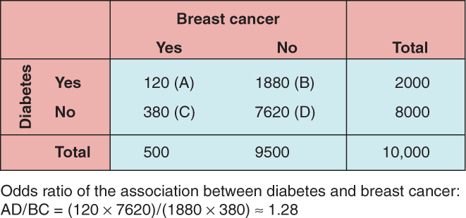
FIGURE 3–9 Results of a hypothetical cross-sectional study evaluating the relationship between the prevalence of diabetes and breast cancer.

Because cases are not necessarily newly diagnosed and may include subjects who have had their disease for many years, cross-sectional studies are sometimes referred to as prevalence studies. The main drawback for this design is that it introduces survival (or prevalence) bias into the study. A factor found to be more prevalent in cases than controls may not be causally related to the onset of disease but instead may be related to living with the disease, its survival, its treatment, or other factors after diagnosis. In the example above, it is likely that having a diagnosis of breast cancer results in increased physical and emotional stress (eg, from surgical procedures, psychosocial stress, or stress that leads to an increase in poor eating habits). In this fashion, subclinical or borderline diabetic patients can become fully diabetic, as a result of these stressors. Second, patients who are diagnosed with breast cancer will see their doctors more often, and have more tests run, including standard blood work. This act can increase the detection of borderline or mild cases of diabetes disproportionate to the general healthy population. Third, some breast cancer chemotherapies are concomitantly administered with steroids (either to prevent anaphylactoid reactions or as a prophylactic antiemetic), which can further push a subclinical or borderline diabetic into being a clinically apparent diabetic.

In another example, the relationship of severe emphysema and early stage lung cancer is examined, using a cross-sectional study design. We may find, paradoxically, that emphysema appears to protect against development of early stage lung cancer. However, the reason for this finding may be a result of emphysema patients dying earlier after diagnosis of lung cancer, or as a result of suboptimal therapy (emphysema patients may not be able to tolerate standard lung resection, or may develop more life-threatening complications after resection). Alternatively, severe emphysema may be such a significant comorbidity that in the presence of a second cause of pulmonary compromise (eg, lung cancer), there is an increase in pneumonia, bronchitis, or general debilitation, and a higher rate of death. Under these circumstances, in a prevalence or cross-sectional study, a substantial proportion of individuals who have lung cancer with severe emphysema may have died by the time of the cross-sectional sampling, and distort the relationship between lung cancer and emphysema, known as survival bias (see Table 3–1). In such circumstance, other study designs, such as case-control or cohort, which typically restrict cases to those who are newly diagnosed, are more appropriate.

Cross-sectional study designs are most useful when studying prevalence questions, such as with health and economic policy research (eg, How commonly are prostate cancer and dementia found together? How many breast cancer survivors are there who are overweight?). Many cross-sectional studies utilize routinely collected information for other reasons (eg, census data) and thus it can be of low cost to perform such secondary analyses. It is less common to have a prospectively designed cancer cross-sectional study, primarily because of the potential for the biases listed above, and the relatively large numbers of individuals (and associated expense) required for completing such a study.

3.4.5 Familial Design

Familial studies are commonly used to study the association of genetic factors with disease risk (Thomas, 2004). Initially family-based studies involved either using sibling pairs, generally one affected and one unaffected sibling, or a single affected offspring and 2 parents. The first can be analyzed using methods related to those used in case-control studies. The latter uses the transmission disequilibrium test, which compares parental alleles to those of the diseased offspring (case) and determines if there is excess transmission of specific alleles to the offspring. Newer statistical methods allow for analyses using families with affected individuals and 1 or more siblings, parents, or combinations of both (Thomas, 2004). The advantage of family based designs over a case-control design is that they are not subject to bias because of the presence of a systematic difference in allele frequencies between subpopulations as a result of different ancestry (known as population stratification). Bias occurs when such a systematic difference goes unrecognized, leading to potential genetic associations that are thought to be related to the disease of interest, but are, in reality, associated with genetic differences arising from individuals having different ethnic backgrounds.

A major difficulty of family based studies is recruitment of controls. If the diseased subject is older, parents may be deceased or not well enough to join a study. Recruitment of siblings can also be difficult as a subject must have a sibling willing to enroll in the study to be eligible. For these reasons familial study designs are rarely employed in cancer outside of a pediatric population. Instead, study designs in adult cancers generally rely on case-control studies where controls are matched to cases for ethnicity and statistical methods are employed to control for population stratification.

3.5 CANCER EPIDEMIOLOGY IN ACTION: SUCCESS STORIES

3.5.1 Infection and Cancer

There has been increasing recognition of the role of infection in cancer etiology. Specific examples include schistosomal infestations and bladder cancer, hepatitis viruses and hepatocellular carcinoma (HCC), and HPVs and cervical and head and neck cancer (see Chap. 6, Sec. 6.2.3). It has been estimated that attributable risk of all cancers worldwide to infections is approximately 18%, and that by reducing the effects of these infectious agents (through improved hygiene and public health measures, vaccination, and sometimes screening), cancer incidence might decrease by 8% and 26% in developed and developing countries, respectively (Parkin, 2006).

One of the most successful applications of analytical epidemiology in addressing infections and cancer is the research that helped establish a role for Epstein-Barr virus (EBV) in the etiology of Burkitt lymphoma (see Chap. 6, Sec. 6.2.4). Endemic Burkitt lymphoma occurs in children, primarily in equatorial Africa and Papua New Guinea. Its occurrence was first described by Dennis Burkitt in 1958 (Thompson and Kurzrock, 2004). The most frequent presentation of the tumor is a distinctive lesion of the jaw. In early ecological studies of this disease, this information was circulated to medical units in Africa and presence of the lesion was mapped to geographic location. Results indicated an association between the presence of Burkitt lymphoma and low-lying areas in tropical Africa (Burkitt, 1962a,b), suggesting that a virus transmitted by an insect vector might play a role in the etiology of this cancer. Laboratory-based studies by Epstein, Achong, and Barr implicated EBV as an etiological agent for this cancer and following further research, EBV became the first virus to be clearly implicated in the development of a human cancer (Thompson and Kurzrock, 2004). Additional research indicates that malarial infections, which correlate with the incidence of Burkitt lymphoma, may interact with EBV to increase risk of Burkitt lymphoma (Brady et al, 2007).

The evidence associating HBV and HCC was first observed in ecological studies, where a high prevalence of serum hepatitis B surface antigen (HBsAg) positivity was correlated with the high prevalence of HCC (Maupas and Melnick, 1981). Cohort studies also showed that populations receiving vaccination for HBV have much lower risk of developing HCC then those without vaccination (Lee et al, 1998). HCV was also identified as an etiological factor, both as a cofactor and an independent risk factor for HCC (Yu et al, 2005). Nowadays, HBV and HCV vaccination is routinely administered in high-prevalence regions, and has substantially reduced the incidence of HCC by 75% in school-age children in the last 2 decades (see Chap. 6, Sec. 6.2.5; Chien et al, 2006).

The association between HPV and cervical cancer was first proposed by zur Hausen in 1977 when he found HPV DNA in cervical cancer tissues (zur Hausen, 1977). In 1995, a large cross-sectional study by the International Agency for Research on Cancer (IARC) reported HPV DNA, predominately HPV types 16 and 18, in 93% of the cervical tumor samples, thus providing strong epidemiological evidence of the association (Bosch et al, 1995). Now HPV is accepted as a necessary cause of cervical cancer; however, only a small portion of the HPV carriers develop cervical cancer, suggesting that other etiological factors are involved (Munoz et al, 2003). In 2006, the first HPV vaccine was approved by the U.S. Food and Drug Administration (FDA) (Markowitz et al, 2007) and HPV vaccine is now recommended in the United States and Canada for school-age girls to prevent cervical cancer (see Chap. 6, Sec. 6.2.3).

3.5.2 Tobacco and Cancer

Tobacco consumption is the most recognized risk factor for human cancer in Western countries. It accounts for approximately 30% of cancer death in the United States (CDC, 2002), and 16% worldwide (Parkin et al, 1999). Epidemiological studies have identified numerous detrimental health effects of tobacco consumption over the last 60 years, with the most striking example being Sir Richard Doll’s British studies that established the association between tobacco smoking and lung cancer (Doll et al, 2004). Since then numerous epidemiological studies have been conducted for different cancer sites. In 2004, an IARC monograph stated that there is sufficient evidence to conclude that in humans tobacco smoking causes cancer of the lung, head and neck (including oral cavity, oropharynx, and larynx), esophagus, stomach, pancreas, liver, kidney, bladder, cervix, and myeloid leukemia (Fig. 3–10) (IARC, 2004). In addition to adult cancers, it is recognized that parental tobacco smoking in the time period just before conception or during pregnancy is associated with a higher risk of hepatoblastoma in the offspring (Secretan et al, 2009).

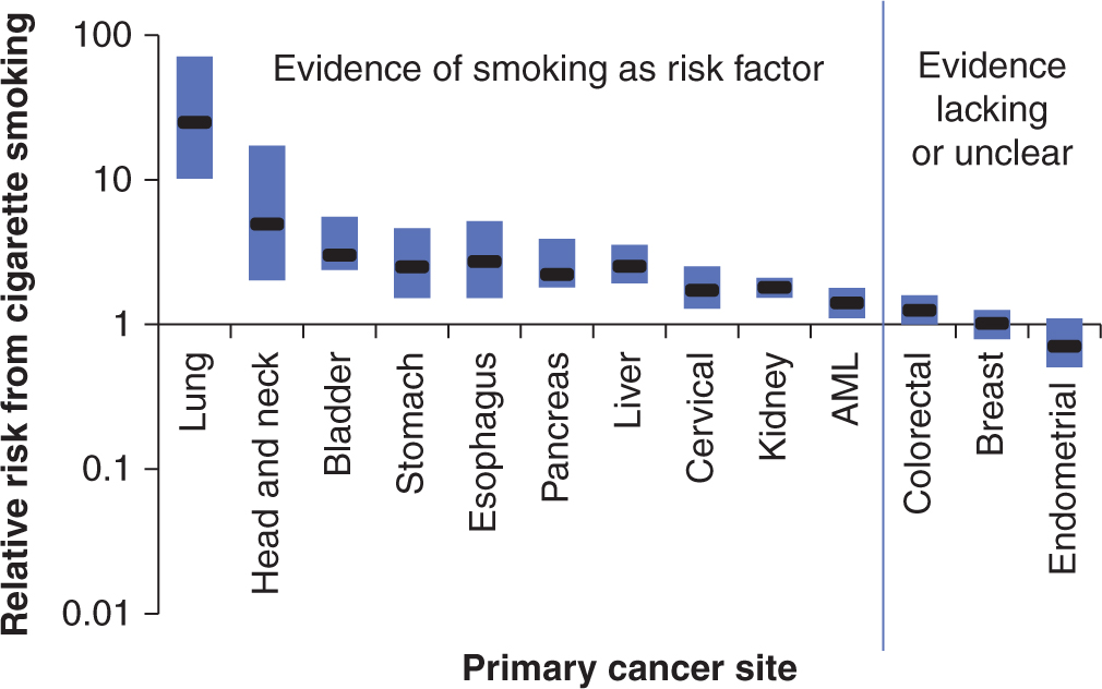
FIGURE 3–10 Relative risks of cigarette smoking on risk of various cancers. The approximate ranges of the relative risks of the heaviest cigarette smokers for developing various cancers, summarized from the tables of published studies reviewed by the International Association for Research in Cancer (IARC). The X-axis indicates various primary cancers. The Y-axis is the median relative risk on a logarithmic scale. The cancers to the left of the blue line were concluded by IARC to have an association with cigarette smoking, while the ones on the right did not. These ranges represent the majority of primary smoking data up to the year 2004. The heaviest smokers were defined variably by different studies. Outlier studies were not included in these ranges, but data for men and women were considered together. The median values are presented in black and the bars represent 25% and 75% quartiles. AML, Acute myelogenous leukemia. (Data from IARC Monograph on Tobacco and Involuntary Smoking, 2004.)

Data for lung cancer are overwhelming: 88% of male lung cancer and 72% of female lung cancer is attributable to tobacco use. Increasing intensity of cigarette smoking (ie, number of cigarettes per day) and increasing duration of smoking (ie, years) are both associated with increasing risk of lung cancer in a dose-dependent fashion. Increasing number of years since smoking cessation is associated with a fall in risk. Similar dose-dependent findings have been found for the risk of bladder, oral cavity, and other solid tumors. There have been more than 50 studies of second-hand smoking and lung cancer risk, many in lifetime never-smoking spouses. Most, especially those associated with higher second-hand smoking exposures, have shown significant increased lung cancer risks associated with inhaling smoke from others (IARC, 2004).

The understanding of the association between tobacco use and cancer risk (in addition to other nonmalignant diseases such as cardiovascular disease) through epidemiological studies have helped governments to implement policy for tobacco control, including banning smoking in public buildings, increasing tobacco taxes, and placing warning labels on the packaging. Government intervention and control policy have helped to reduce tobacco consumption at the population level substantially, and to reduce cancer deaths related to tobacco consumption.

3.5.3 Alcohol and Head and Neck Cancer

Epidemiological studies have found an association between alcohol consumption and cancer at various sites, including cancers of the oral cavity, pharynx, larynx, esophagus, liver, female breast, and colorectum (IARC, 2010). The role of alcohol as a causative factor for other cancers, such as lung cancer and non-Hodgkin lymphoma, is inconclusive. A systematic review estimated that alcohol accounts for 5.2% of overall cancer worldwide in males and 1.7% in females (Boffetta and Hashibe, 2006). Studies have also investigated the dose–response relationship between alcohol consumption and cancers, and the synergism between alcohol and tobacco smoking. Because alcohol is often consumed by tobacco smokers, there was a need to take tobacco smoking into account either by study design or statistical analysis to address potential confounding. The dose–response relationship between alcohol and head and neck cancers was shown to be linear with an approximately 2- to 3-fold increased risk per 50 g of alcohol per day, depending on the cancer site (IARC, 2004). The effect of smoking and alcohol consumption appear to be multiplicative for head and neck cancer, showing a synergistic interaction between these 2 factors (see Fig. 3–8).

3.6 EMERGING AREAS IN EPIDEMIOLOGY

3.6.1 Genomic Epidemiology

3.6.1.1 Genome-Wide Association Studies Genome-wide association studies (GWAS, see Chap. 2, Sec. 2.7) aim to investigate the majority of genetic variations across the genome, and do not require prior knowledge of the functional significance of the variants studied. They are used increasingly to discover susceptibility genes in various health research domains. Genome-wide scans for cancer of the prostate, breast, colon, lung, kidney, bladder, and pancreas have been completed, and this approach has been successful in identifying cancer susceptibility loci. A catalog of published GWAS with complete references is maintained by the National Human Genome Research Institute (available at http://www.genome.gov/gwastudies/).

3.6.1.2 Addiction to Nicotine, and Risk of Lung Cancer A previous linkage analysis of 52 high-risk pedigrees identified a lung cancer susceptibility locus at chromosome 6q23-25 (Bailey-Wilson et al, 2004), but specific genetic factors that influence lung cancer susceptibility were not defined until the GWAS findings were reported in 2008, when researchers identified the susceptibility loci at 15q25 and 5p15 (Hung et al, 2008). The Ch15q25 region is comprised of several nicotinic acetylcholine receptor genes and the 5p15 region includes the genes hTERT (see Chap. 5, Sec. 5.7) and CLPTM1L. The hTERT gene is the most likely candidate in this region. The Ch15q25 region was also shown to be associated with nicotine addiction and smoking behaviors (Thorgeirsson et al, 2008), although the association between 15q25 and smoking is not sufficient to explain its strong association with risk of lung cancer. Alternative hypotheses relating to potential roles in angiogenesis and in the repair of epithelium are being evaluated. This example illustrates how GWAS may contribute to the understanding of cancer etiology. As yet, none of the findings from GWAS is of strong enough magnitude to translate into the clinical setting; hence, GWAS is still a research tool used to identify novel biological pathways for further basic and translational research.

3.6.1.3 Alcohol, Alcohol Dehydrogenase, and Head and Neck Cancer The metabolism of alcohol mainly involves two families of genes: alcohol dehydrogenases (ADHs) that oxidize ethanol to acetaldehyde, and acetaldehyde dehydrogenases (ALDHs) that further metabolize acetaldehyde to acetate. The genetic variation of ADHs and ALDHs that influences enzyme activity has been investigated for their association with head and neck cancer in several epidemiological studies (IARC, 2010). ADH1B (*1/1, where *1/*1 is a genotype designation) and ADH1C are associated with increased risk of head and neck cancers, although the mechanism has not been elucidated. The ALDH2 Glu487Lys allele (rs671, also known as *2 variant allele) encodes an inactive form of the enzyme, and this Lys variant is prevalent in approximately 30% of Asian populations. The heterozygous carriers have approximately 10% enzyme activity, and they accumulate acetaldehyde and have increased risks for alcohol-related esophageal and head and neck cancers compared with individuals with the common alleles. These findings have contributed to the understanding of alcohol as a carcinogen (IARC, 2010).

3.6.2 Pharmacogenomic Epidemiology and Pharmacoepidemiology

Pharmacogenomic epidemiology is focused on personalizing medicine through the evaluation of tumor and germline (heritable) genetic and genomic factors to select appropriate and individualized therapies, through the use of epidemiological tools. These factors, or biomarkers, are assessed for their association with pharmacokinetic and pharmacodynamic roles in affecting treatment response, recurrence, disease progression and survival, and toxicity of treatment (see Chap. 18, Sec. 18.1).

The classical example in cancer pharmacogenetics has been the genetic disorder that results in the complete absence of functional dihydropyrimidine dehydrogenase (DPD), or DPD deficiency, and the resultant severe hematological and gastrointestinal toxicities that affect such patients who receive fluoropyrimidines (eg, 5-fluorouracil), which are antimetabolites that inhibit thymidylate synthase and DNA synthesis (see Chap. 18, Sec. 18.1.3). DPD is the enzyme responsible for more than 85% of the inactivation and metabolism of 5-fluorouracil. However, the cause of this rare syndrome of DPD deficiency is multifactorial, including such factors as multiple functional genetic variants within the DPD gene, and both genetic and epigenetic regulation across other related pathway genes that secondarily alter DPD function. Pharmacological factors (drug–drug interactions) are also being evaluated. Thus, the original single defect in 1 gene leading to a single phenotype is too simplistic a model to explain sensitivity to fluoropyrimidines. Additional factors also explain the low positive predictive value of currently available tests; as such, routine clinical testing is generally not recommended. Because of the rarity of DPD deficiency, pharmacoepidemiological (pharmacovigilance) studies have been used to identify potential cases, and these are matched, in a case-control design, to appropriate controls (patients receiving the drug who suffered no significant toxicity).

Several newer pharmacogenetic studies have identified promising associations between heritable genetic variations and either toxicity or efficacy of drugs (Table 3–4). Each of these studies has either used observational methods or involved secondary analyses of randomized clinical trials. Some have selected candidate polymorphisms (eg, of genes known to be important in metabolism of anticancer drugs), whereas others have utilized GWASs without a primary hypothesis. These studies have led to the discovery of unexpected genetic variants that have a biological rationale for their association with the pharmacogenetic effects. Validation studies are ongoing.

TABLE 3–4 Examples of cancer pharmacogenetic studies.

In addition to heritable genetic associations with drug therapy, molecular epidemiological studies and secondary analyses of randomized controlled trials are also demonstrating associations between tumor markers and treatment outcomes. Four examples are: estrogen receptor/progesterone receptor status and use of antiestrogen therapy (eg, tamoxifen or aromatase inhibitor; see Chap. 20, Sec. 20.4.1); KRAS mutation predicts lack of efficacy of monoclonal antibody therapy targeting EGFR in colorectal cancer (see Chap. 17, Sec. 17.3.1); Her2/neu overamplification predicts efficacy of monoclonal antibody therapy targeting Her2/neu (see Chap. 20, Sec. 20.3.3); and EGFR mutation predicts for response to small molecule inhibitors of EGFR (see Chap. 17, Sec. 17.3.1).

3.7 ISSUES AND CHALLENGES IN CANCER EPIDEMIOLOGY

3.7.1 Observational Studies Versus Clinical Trials, Predictive Versus Prognostic Biomarkers

Observational studies are the most common way to study the risk of disease, primarily because there are generally no other approaches available. Observational studies are also a useful source of data for certain outcomes analyses.

Randomized clinical trials provide a convenient source of patients for analysis of disease outcome and may be linked to biospecimens. When available, they can be used sometimes for secondary analyses of factors other than the one that was randomized. Randomized clinical trials are a form of cohort study where subjects are assigned to 2 or more arms (eg, vitamin supplementation group and placebo group) and the cohort is followed over time. Unlike modern observational cohorts, randomized trials typically focus largely on a single factor. Their main advantage is that the researcher controls who is exposed to the potential disease-related factor, through random assignment. Randomized trials are most useful in clinical medicine for demonstrating effectiveness of a specific treatment intervention (see Chap. 22, Sec. 22.2.3).

When molecular factors are evaluated that might predict response, toxicity, or outcome related to the experimental therapy used in a randomized trial, a pharmacogenomic analysis takes place. A major benefit of performing a secondary analysis of a randomized trial is that one can determine whether the pharmacogenomic factor is predictive of treatment response or simply a general prognostic marker (see Chap. 22, Sec. 22.4). Predictive biomarkers are those that are associated with a specific therapy; in the absence of this therapy, the biomarker is either no longer associated with outcome, or is associated in a different manner. The absence of a differential effect by treatment implies that the specific biomarker is a general prognostic factor. Although prognostic factors may be helpful for improving our understanding of cancer biological pathways, they are less useful clinically than biomarkers that predict whether an outcome will change if a specific treatment is given. The predictive biomarker can then direct the choice of therapy, in essence, personalizing the treatment. Because the only way to determine whether a biomarker is predictive is to have a control arm, a randomized trial is optimal for identifying such predictive pharmacogenomic biomarkers.

The formal statistical method for determining whether a marker is predictive is to identify an interaction between a biomarker and a treatment arm. The presence of such an interaction implies that the biomarker has a different effect in the presence of the treatment than in the absence of treatment. Although observational studies may occasionally be used to study such interactions (Bradbury et al, 2009), randomized trials offer the best opportunity, partly because the choice of therapy is less confounded by other key prognostic variables such as patient co-morbidity.

Table 3–5 compares the use of randomized trials with observational studies. A randomized trial of the right set of patients may not be available (wrong patient subgroup, wrong therapy, rare cancer type where no such randomized trials are being conducted), and an observational study becomes the only option. Thus, both types of studies will continue to be important for epidemiological and translational research. Figure 3–11 details the long journey from biomarker discovery through to clinical adoption. Epidemiological studies are key to several of the steps in the biomarker developmental pipeline.

TABLE 3–5 Comparing the advantages and disadvantages of using randomized trials versus observational studies as sources of epidemiological analyses.

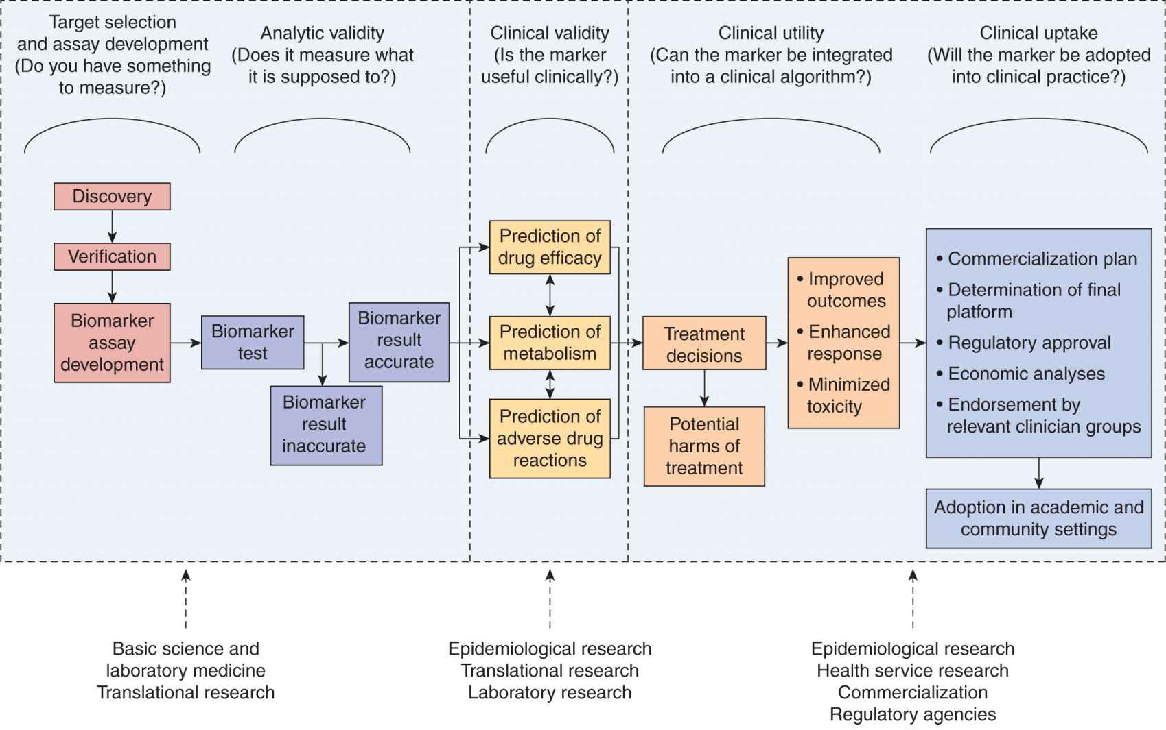
FIGURE 3–11 The long road from biomarker discovery to clinical use, and where epidemiological studies play a key role.

3.7.2 Exposure Misclassifications: The Example of Diet and Occupation

As discussed briefly in Section 3.2.4, misclassification of exposure has been a challenge for cancer epidemiology, and specific examples include assessment of dietary and occupational exposures. The general hypotheses are that certain micro-nutrients or specific chemical agents related to occupations can affect cancer risk. Proper assessments of these exposures require a comprehensive study protocol, thorough validation, and substantial resources.

For dietary exposures, specific instruments, such as 24-hour recall, have been developed to assist the validation of the self-reported dietary history. To validate a specific dietary exposure, biochemical indicators (if available) might be measured, such as serum level of vitamin B or folate. This approach, however, is subject to biomarker instability, laboratory measurement error, and when repeated samples are not available, the measurement at 1 time point does not reflect the long-term exposure history. Nevertheless, biomarkers can provide qualitative information regarding the validity of information obtained from questionnaires.

Perhaps the greatest challenge in evaluating exposure to putative risk factors is the problem with highly correlated exposures, where the challenge is to distinguish the independent effect of specific nutrients or foods, when food items are typically consumed in groups, and patterns of consumption are reflective of general lifestyle and socioeconomic status. An individual food item might be a better unit for analysis because it can be directly related to dietary recommendations and the same nutrients may exhibit different properties in different foods (eg, nitrates in smoked meat versus in green leafy vegetables). Analysis based on a specific nutrient can be more directly related to a biological mechanism and avoid the issues of interrelated dietary behavior patterns (eg, the tendency to eat certain foods together, such as milk and cereal, or certain habits together such as alcohol and tobacco consumption). In general, it has been suggested that maximum information can be obtained when analyses are performed using all of the data, including nutrient levels, food items, and food groups.

The approach of Mendelian randomization has also been proposed to address the issues of complex exposures (Smith and Ebrahim, 2003). The basic concept of Mendelian randomization is to analyze variants in genes (both as single genes or multiple genes) that determine metabolism of nutrients as instrumental (ie, surrogate) variables for the specific nutrients of interest, as genetic alleles are randomly assorted in the population based on Mendel’s laws and their assortments are unrelated to other factors such as lifestyles or other food intake. Specific examples include ALDH (for alcohol consumption) and cardiovascular disease, or lactase persistence genotype (for milk consumption) and cancer (Smith and Ebrahim, 2003). The ideal instrumental variable needs to have very strong and specific correlations with the nutrient of interest, but for some nutrients, such an instrumental variable will not be found. Nevertheless, it provides a potential alternative solution to the issues of misclassification and high correlation in nutritional epidemiology.

3.7.3 High-Dimensionality Data and Multiple Comparisons

Biological and genetic data from cancer epidemiological studies typically involve tens or hundreds of thousands of variables related to genetics or biomarkers to be tested against a null hypothesis. If we conduct 100 independent tests each with 95% confidence interval (5% type I error rate, see Chap. 22, Sec. 22.2.5), we would expect to reject the null hypothesis for 5 tests as a result of chance. This is the result of multiple comparisons. The conventional approach to address the issue of multiple comparisons is to alter the level of significance by dividing it by the number of comparisons, known as the Bonferroni method. For example, one would use a type I error rate of 0.05/100 = 0.0005 for 100 simultaneous comparisons. However this approach has various limitations, such as a naïve global null hypothesis that ignores prior knowledge about biological effects and low efficiency, and it is deemed to be too conservative for epidemiological investigation. Analogous to Bayesian statistical models that incorporate prior information (see Chap. 22, Sec. 22.3.5), modern approaches, such as hierarchical modeling or mixture modeling, can offer improved performance over the Bonferroni adjustment. These analytical approaches are being applied to the field of genomic and molecular epidemiology (Chen and Witte, 2007). The details of these modeling approaches are beyond the scope of this chapter, but the basic concept of hierarchical modeling is to incorporate prior knowledge of markers into analysis through a prior matrix of quantitative weighting factors (Hung et al, 2007) These weighted factors will be used to “adjust” for the biological and genetic results, thereby improving the potential for finding true positive associations.

3.7.4 Analyses across Multiple Studies

To integrate evidence from multiple studies, approaches such as pooled analysis and metaanalysis (see Chap. 22, Sec. 22.2.7) are being increasingly applied in cancer epidemiology. Meta-analysis is typically based on published results; thus, it is susceptible to publication bias, and then limited to results reported in the publication and subject to the definition of different variables and covariate adjustments. It is often impossible to conduct detailed analysis for specific subgroups using meta-analysis. Consequently, researchers have started to conduct pooled analysis to address the above limitations by combining individual-level data from different studies, analogous to patient-based metaanalysis of therapeutic trials. More detailed analysis can also be conducted for specific subgroups. The methodology of metaanalysis and pooled analysis is described elsewhere (van Houwelingen et al, 2002). To facilitate this type of pooled analysis, several cancer consortia have emerged, including the International Lung Cancer Consortium, the Breast Cancer Association Consortium, the Pancreatic Cancer Case-Control Consortium (Ioannidis et al, 2005). The growing list of cancer consortia can be found at http://epi.grants.cancer.gov/Consortia/. The same website lists consortia publications that replicate initial findings in the post-GWAS era, showing that such consortia are an efficient way to replicate an initial finding and provide further evidence for supporting or disputing an observed association.

SUMMARY

• Epidemiology is the study of the distribution and determinants of disease and disease outcomes in human populations. It is complementary to basic and translational research.

• Epidemiological methods can be descriptive or analytical:

Descriptive studies provide information about populations and their distributions, including distributions of disease determinants.

Analytical studies assess associations between disease determinants and disease and disease outcomes and include case-control, cohort, cross-sectional, and familial designs.

• Important epidemiological successes have demonstrated the relationships between various infections (HPV, viral hepatitis, EBV) and cancer risk, tobacco and cancers, and alcohol and head and neck cancer.

• Emerging areas in epidemiology include genomic epidemiology, and pharmacoepidemiology.

• Challenges for the future include:

Utilizing secondary analyses of clinical trials.