2.1 Introduction
Nutritional epidemiology is the application of epidemiological techniques to the understanding of disease causation in populations where exposure to one or more nutritional factors is believed to be important. Epidemiology aims to:
- describe the distribution, patterns and extent of disease in human populations
- understand why disease is more common in some groups or individuals than others (elucidate the etiology of disease)
- provide information necessary to manage and plan services for the prevention, control and treatment of disease.
Much of the focus of nutritional epidemiology has been on the elucidation of the causes of chronic disease, especially heart disease and cancer. However, the onset, development and expression of these diseases are complex, and the role of diet in the initiation of disease may be different from its role in the progression of disease. The dietary factors that contribute to the occlusion of an artery may not be the same factors that increase the acute risk of myocardial infarction. Disentangling these complex relationships is one of the aims of nutritional epidemiology.
Another important function of nutritional epidemiology is to evaluate the quality of the measures of exposure or outcome that are made. It is notoriously difficult to measure exactly how much food people eat or to determine the nutrient content of the diet. Determination of the severity of disease (e.g. the degree of blockage in the arteries of the heart) and measurements of physiological states (e.g. blood pressure) are also subject to inaccuracies. Extensive misclassification of exposure or outcome in an epidemiological study will seriously undermine the ability to determine diet– disease relationships.
A key purpose of nutritional epidemiology must be to inform public health nutrition, a population approach to the prevention of illness and the promotion of health through nutrition. Public health nutrition puts nutritional epidemiological findings into a wider social and ecological context to promote “wellness” through a healthy lifestyle, including good diet. A glossary of terms used in nutritional epidemiology is presented in Box 2.1.
| Term | Definition |
| bias | Deviation of results or inferences from the truth, or processes leading to such deviation. Any trend in the collection, analysis, interpretation, publication or review of data that can lead to conclusions that are systematically different from the truth |
| case–control study | An epidemiological study that starts with the identification of persons with the outcome of interest and a suitable control group of persons without the disease. The relationship of an exposure to the outcome is examined by comparing the group with the outcome to the control group, with regard to levels of the exposure |
| causality | The relating of causes to the effects they produce. Causality may defined as “necessary” or “sufficient”. Epidemiology cannot provide direct proof of cause, but it can provide strong circumstantial evidence |
| cohort study | An epidemiological study in which subsets of a defined population have been or may be in the future exposed to a factor hypothesized to be related to the outcome of interest. These subsets are followed for a sufficient number of person-years to estimate with precision, and then compare, the rates of outcome of interest |
| confounder or confounding variable | A variable that can cause or prevent the outcome of interest, is not an intermediate variable, and is associated with the factor under investigation |
| cross-sectional study | A study in a defined population at one particular period that investigates the relationship between health characteristics and other variables of interest |
| crude death rate | A crude rate is a simple measure for the total population. The crude death rate for a given year is the number of deaths in that year divided by the midyear count of the population in which the deaths occurred |
| ecological fallacy | The bias that may occur because an association observed between variables on an aggregate level does not necessarily represent the association that exists at an individual level |
| effect modifier | A factor that modifies the effect of a putative causal factor under study |
| exposure | Factor or characteristic that is a presumed determinant of the health outcome of interest |
| incidence | The number of new outcome events in a defined population during a specified period. The term incidence is sometimes used to denote incidence rate |
| incidence rate | Expresses the force of morbidity in a cohort of persons while they are free of the outcome. It is the number of new events during a defined period, divided by the total person–time units of experience over the period |
| misclassification | The erroneous classification of an individual, a value or an attribute into a category other than that to which it should be assigned. The probability of misclassification may be the same in all study groups (nondifferential misclassification) or may vary between study groups (differential misclassification) |
| morbidity | Any departure, subjective or objective from a state of physiological or psychological well-being |
| mortality | Death |
| odds ratio | An approximation of relative risk based on data from a case–control study |
| outcome | Identified change in health status |
| period prevalence | The total number of persons known to have had the disease or attribute (outcome) at any time during a specified period |
| person-years at risk | A unit of measurement combining person and time (years), used as a denominator in incidence rates. It is the sum of individual units of time (years) that the persons in the study have been exposed to the condition of interest |
| point prevalence | See prevalence |
| population | A defined set of units of measurement of exposure or outcome. The members of a population can be individuals or experimental units, e.g. schools, hospitals, doctor’s surgeries, towns, countries |
| prevalence | The number of instances of a given outcome in a given population at a designated time (specified point in time) |
| quality-adjusted life-years | The product of length of life and quality of life score. A measure of the length of life or life expectancy adjusted for quality of life |
| quality of life | Quality of life may be used as a global term for all health status and outcomes including objective and subjective outcomes. In specific use it is an evaluation of one’s position in life according to the cultural norms and personal expectations and concerns, and thus is inherently subjective |
| rate | A rate is a ratio whose essential characteristic is that time is an element of the denominator. In epidemiology, the numerator of the rate is all cases or outcome events derived from the population at risk, during a given period. The denominator is the population at risk, as defined for the same period |
| ratio | The value obtained by dividing one quantity by another |
| relative risk | The incidence of disease (or other health outcome) in those exposed to the risk factor under investigation divided by the incidence of disease in those not exposed |
| sample | A sample is a selection of items from a population. It is normal practice to make the sample representative of the population from which it is drawn |
| sampling frame | A list of the items in a population from which a sample can be drawn |
Historical context
The history of nutrition as a science dates back just over 100 years. The history of nutritional epidemiology is even shorter. Observations of associations between diet and health date back to Greek times. In 1753 James Lind observed that British sailors who took fresh limes on long sea voyages escaped the ravages of scurvy, at that time a common cause of morbidity and mortality. This observation led to changes in practice (and the epithet “limeys” for British sailors). Systematic observation of populations did not become common until the mid-nineteenth century, and then focused more on infective than on chronic disease.
The understanding of the role of nutrients in deficiency disease gained ground early in the twentieth century with the discovery of vitamins and the acceptance that a lack of something in the diet could be a cause of ill-health. It was not until the second half of the twentieth century that an understanding of the role of exposure in chronic disease became well established, mainly through the model of smoking and lung cancer. In addition, complex multifactorial models of causation became better accepted. Statistical techniques and the advent of computers added a further boost to these disciplines by facilitating the disentanglement of complex exposures which often included causal elements that were correlated or that interacted. For example, the effects of vitamin C and other antioxidant nutrients on the risk of heart disease were difficult to disentangle from the effects of smoking, because smokers typically consume diets with lower levels of antioxidants and smoking itself increases the requirement for antioxidants.
A further boost to nutritional epidemiology was the clarification of the ways in which measures of dietary exposures were imperfect. What a person reported in an interview or wrote down about their consumption was not necessarily the truth. It had been recognized that confectionery and alcoholic beverages were regularly underreported (comparison of average consumption based on national surveys of individuals and national sales figures typically show two-fold differences). Other, more subtle misreporting of consumption took much longer to come to light. This was particularly true in the case of people who were overweight and who, on average, underreported their food consumption. This recognition of underreporting was one factor that helped to explain why the association between fat consumption and heart disease was observed internationally but not at the individual level. This issue of misclassification is discussed in detail in Section 2.4.
The most recent development in nutritional epidemiology has been the inclusion of genetic risk factors in models of causation. Genetic influences work in two ways: genes influence the ways in which nutrients are absorbed, metabolized and excreted; and nutrients influence the ways in which genes are expressed. It will be a challenge over the next 50 years to elucidate the role of nutrition-related genetics in the etiology of disease.
Measurements of exposure and outcome and how they relate
The aim of most epidemiological studies is to relate exposure to outcome. The epidemiologist must define exactly which aspects of exposure and outcome are believed to be relevant to disease causation or public health. In nutritional epidemiology, there will be a chain of events starting with the diet and ending with ill-health, disease or death. The principal tasks of the nutritional epidemiologist are to decide which aspect of dietary or nutritional exposure is relevant to the understanding of causation, and to choose a method of measurement that minimizes misclassification.
For some diet–disease relationships, this may be relatively straightforward. If there is a deficiency of a single nutrient (e.g. iodine) that is strongly and uniquely associated with an adverse outcome (cretinism in the offspring of iodine-deficient mothers), only one set of measurements will be required. Iodine intake, for example, can either be measured directly by collecting duplicate diets, or estimated indirectly by collecting 24 h urine samples (the completeness of which needs to be established). It is then possible to identify a threshold for iodine intake below which the risk of an adverse outcome increases dramatically.
Exposures relevant to the causation of heart disease or cancer, in contrast, are enormously complex. Not only is there a large number of possible dietary influences (energy intake in relation to energy expenditure, total fat intake, intake of specific fatty acids, intake of antioxidant nutrients, etc.), but different nutrients (and non-nutrients) will have different influences on disease initiation, progression and expression at different points in time. Moreover, many important non-nutritional influences (e.g. smoking, blood pressure, activity levels, family history/genetic susceptibility) will need to be taken into account when analyzing the results, and some of these factors (e.g. smoking and blood pressure) will have links to diet (e.g. high calcium intakes are associated with lower blood pressure, smoking increases the body’s demand for antioxidant nutrients).
Causality
Central to the understanding of how diet and health outcomes relate to one another is the notion of causality. Epidemiology deals with associations, analyzing their strengths and how specific they are. Thus, nutritional epidemiology does not establish cause per se, but it can provide powerful circumstantial evidence of association.
Causality is often categorized as necessary or sufficient. Most communicable diseases, for example, have a single identifiable cause (a pathogenic bacterium or virus) that is responsible. Thus, it is both necessary (i.e. it must be present) and sufficient (no other factor is required). However, people do not catch a cold every time they are exposed to a cold virus. This is because other factors influence the ability of the virus to mount a successful attack. These include the state of the immune system, which in turn depends on a person’s general health and (in part) their nutritional state.
A more complex example would be the risk of developing lung cancer. Smoking increases the risk, but not everyone who smokes develops lung cancer, and there are people who develop lung cancer who have never smoked. Thus, smoking may be sufficient but is not strictly necessary. There are other factors that can cause lung cancer (e.g. exposure to asbestos) and factors that may protect against the damage caused by smoking (e.g. a high intake of antioxidant nutrients).
Hill was the first to set out a systematic set of standards1 for causality. Others have since elaborated Hill’s work. The following have been considered when seeking to uphold causality.
Strength
Strong associations are more likely to be causal, while the converse is not always true (weak associations are non-causal). For example, the association between smoking and heart disease; it is more likely that weak associations exist either because of other factors that contribute to the presence of something as common as heart disease, or because there are undetected biases in the measurements that lead to the appearance of a spurious association, or because of confounding. Strong associations may also occasionally be explained by confounding. For example, low intake of fruit and vegetables is associated with short stature in children, but is explained by the effects of social class. “A strong association serves only to rule out hypotheses that the association is entirely due to one weak unmeasured confounder or other source of modest bias.” (Rothman and Greenland 1998.)
Consistency
If the same association is observed in a number of different populations based on different types of epidemiological study, this lends weight to the notion of causality. Lack of consistency, however, does not rule out an association which may exist only in special circumstances.
Specificity
Hill argued that specificity was important (it certainly is in infection), but Rothman and Greenland regard the criterion as having little value in understanding diseases that may have multicausality because one exposure (such as smoking) can lead to many effects.
Temporality
It is presupposed that cause precedes effect. However, circumstances in which the suspected cause is present only after the outcome appears (e.g. markedly raised blood cholesterol levels after a myocardial infarction) do not mean that there may not be a role for the putative factor when measured in other circumstances.
Biological gradient
This is the dose–response criterion: as exposure increases, the likelihood of the outcome increases. Risk of lung cancer increases with the number of cigarettes smoked. Risk of heart disease increases with increased intake of saturated fatty acids. Not all relationship are linear across the range of exposure. Some relationships show a threshold effect: in sedentary societies such as the UK and USA, when calcium intakes exceed 800 mg/day, there is no obvious association with bone mineral density in postmenopausal women, whereas below 800 mg, there is a direct relationship. Even more complex is the J-shaped curve showing that moderate intake of alcohol (10–30 g/day) is associated with a lower risk of heart disease than either no intake or intakes above 40 g/day, where risk increases with increasing intake. Some of the explanation may be due to confounding.
Plausability
There must be a rational explanation for the observed association between exposure and outcome. Lack of a plausible explanation does not necessarily mean, however, that the association is not causal, but simply that the underlying mechanism is not understood.
Coherence
The observed association must not contradict or conflict with what is already known of the natural history and biology of the disease. It is the complement of plausability.
Experimental evidence
This refers to both human and animal experimentation in which the levels of exposure are altered and the changes in the outcome of interest are monitored. More often than not, however, the reason for undertaking an epidemiological study is that the experimental evidence is lacking. This is especially true in nutrition, where long-term exposures that may be responsible for the appearance of disease are virtually impossible to model in an experiment. Thus, the use of experimental evidence to corroborate epidemiological findings is usually limited to short steps in what may be a long and complex causal pathway.
Rothman and Greenland include “analogy” as a final criterion, but its application is obscure. Ultimately, causality is established through a careful consideration of the available evidence. If there is no temporal basis, a factor cannot be causal. Once that is established, however, the causal theory should be tested against each of the standards listed above. It should be kept in mind that confounding may be operating (e.g. children moved from inner cities to the countryside were quickly cured of rickets, supporting the bad air or miasma theories and not the notion of a missing vitamin or exposure to ultraviolet light).
Bias and confounding
Bias is defined by Last as:
Deviation of results or inferences from the truth, or processes leading to such deviation. Any trend in the collection, analysis, interpretation, publication, or review of data that can lead to conclusions that are systematically different from the truth.
Bias can arise because of measurement error, errors in reporting, flaws in study design (especially sampling), or prejudice in the reporting of findings (the more conventional lay use of the term). Last describes 28 different types of bias that can arise. These relate to errors of ascertainment (not selecting a representative group of cases of illness or disease), interviewers (asking questions in different ways from different respondents), recall (how much respondents can remember) and so on. Most researchers work hard to identify likely sources of bias and eliminate them at every stage. Failure to do so will produce information that is misleading.
One of the most important sources of bias is confounding. Confounding bias leads to a spurious measure of the association between exposure and outcome because there is another factor that affects outcome that is also associated with the exposure. For example, there is a strong apparent association between consumption of alcohol and risk of lung cancer. However, people who drink are more likely to smoke, which in turn increases their risk of lung cancer. Thus, in a study of the effect of alcohol intake per se on risk of lung cancer, smoking is a confounding factor. Failure to take into account the effect of smoking will lead to a spurious overestimate of the effect of alcohol intake on the risk of lung cancer.
The two most common confounders are age and gender. Exposure (e.g. diet) changes with age and differs between the genders. Moreover, there are many factors such as hormones, body fatness and health behaviors that differ according to age and gender.
For any given study, the list of confounders may be very long. While it may be possible to match in study design for age and gender, matching may not be feasible for all other confounders. Modern statistical analysis facilitates the control of the effect of confounding. The important issue, therefore, is to make sure that all of the important likely confounders are measured with good precision.
A particular problem in nutritional epidemiological studies is that confounding variables are often measured with greater precision than dietary variables. As a result, there are fewer errors in classification of subjects according to the distribution of the confounding variables than the main dietary variables of interest. In sequential analyses, the apparently significant effects of a dietary factor often disappear when confounding variables are introduced. This may be due to genuine confounding of the dietary factor, or it may be that the effect of the dietary exposure is masked because of the greater precision of measurement of the confounding variable. For this reason, attention to the measurement of errors is critical in nutritional epidemiological studies.
Statistical interpretation and drawing conclusions
One reason that many students do not like epidemiology is the complexity of the statistical analyses and the difficulty of their interpretation. In the most straightforward designs, statistical analysis may be uncomplicated. Suppose that a researcher wanted to investigate the short-term benefit of using a cholesterol-lowering margarine on circulating cholesterol levels. An appropriate group of subjects (e.g. men aged 45–54 years with moderately raised serum cholesterol levels and no history of cardiovascular disease) could be defined; they could be divided into treatment and control groups and asked to consume on average 20 g of the margarine per day (giving them “treatment” margarine in one group and “control” margarine in the second group), and the change in serum cholesterol levels could be measured after 6 weeks. Anaylsis could be by unpaired t-test (if the subjects had not been matched, but the two groups were similar in composition) and a clear conclusion drawn.
Alternatively, if a researcher wanted to investigate the effects of polyunsaturated fatty acid intake on risk of heart disease in a case–control study, also in men aged 45–54 years, conditional logistic regression could be used to determine the odds ratio (the approximation of relative risk) and control for the effects of age, smoking, blood pressure, body size, adiposity, waist/hip ratio (WHR) and other aspects of diet (e.g. dietary fiber, cholesterol, saturated and monounsaturated fatty acids, antioxidant nutrients). How the outcomes are interpreted then depends on the familiarity of the researcher with the ways of expressing the results and the errors likely to arise within the measurements.
2.2 Types of study
Epidemiological studies
The science of epidemiology has taken the statistical tools of experimental design that were developed first in the area of agricultural experiments, and developed formalized systems for inference using other designs. These designs are not experimental, but mimic the principles of experimental design as closely as possible. One key principle is to compare like with like. Another principle is to set up the study so that inferences may be made back to the population from which the study subjects arose (i.e. that the samples are selected so as to make them representative of the population from which they are drawn). These key principles are often referred to as internal and external validity, respectively.
This general philosophy of avoiding bias in the interpretation of an exposure–disease association is put into practice by using appropriate techniques both at the design stage and at the analysis stage in an epidemiological investigation. Careful design can avoid many biases, and other potential biases can be adjusted for or controlled for in the statistical analysis.
The choice of study design is typically dictated by the nature of the research question and progress to date in addressing a particular question. New hypotheses or the search for a hypothesis can often be investigated initially using the ecological approach. Alternatively, a crosssectional study carried out in a representative sample of the population can yield clues to associations. Once there is justification for a particular hypothesis, it is then appropriate to design a careful observational study that uses the principles described above. The choice will depend on the relative ease of constructing groups of people based on their exposure levels or on their disease end-points. If groups are based on exposure, the groups can then be followed forward in time until sufficient disease end-points have accrued (cohort study). If groups are based on end-points, retrospective information on prior exposures is obtained (case–control study).
Ecological studies
Ecological designs are so called because they often take the form of comparing regions of a country with other regions, or countries with other countries. This class of study also includes comparisons over time. Alternative names include indirect studies and population studies. The defining characteristic is that the average exposure for a study unit is compared with an average disease rate. If there is any variation about that average within regions or countries, there is a possibility that those exposed do not overlap with those diseased, in which instance false inferences (known as the ecological fallacy) might be drawn.
Geographical comparisons are often useful for obtaining clues as to the role of dietary factors in disease risk. For example, mortality rates from coronary heart disease and dietary fat calories using countries as data points were examined in several ecological studies. This led to cohort studies of fat and animal fat and coronary heart disease risk. In addition, studies have examined dietary fat and breast cancer mortality, and dietary fat and colon cancer mortality using the ecological method. In a careful study of fish consumption and risk of cardiovascular disease, three different periods were used to study correlations using data from 36 countries. Fish consumption data were obtained from food balance sheets collected by the World Health Organization (WHO) from 1980 to 1982 for each country. Age-standardized mortality rates per 100 000 per year, standardized to 45–74 years of age, were also obtained from the WHO, and averaged for the most recent 3 years. Considerable scatter was found about the regression line, but overall there was a significant inverse association (p < 0.001) between the log-transformation of fish consumption as percentage energy and the log-transformation of all-cause mortality.
Cross-sectional studies
Cross-sectional studies collect information on exposure and outcome from a common period. There is no way to state unequivocally that the exposure preceded the disease (or vice versa). The strongest design in this class is the cross-sectional design that is a census or representative sample from the population.
Cohort studies
Cohort studies are observational epidemiological studies that identify exposures in a defined population (that becomes the cohort), and then follows the cohort through time, identifying outcomes as they occur. They avoid the difficulties of recall bias that are suspected in case–control studies, but are very costly and extremely inefficient as a method for studying rare outcomes.
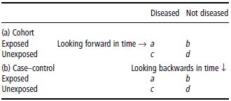
In a cohort study, subjects are measured at baseline for exposure to factors thought either to promote or to protect against disease (Table 2.1a). The subjects are then followed up over time. Naturally, not everyone who is exposed to the factor develops the disease. Conversely, some people who have not been exposed will get the disease. The incidence of disease in the exposed group is then compared with the incidence in the unexposed group. The comparison of the rates is known as the relative risk (RR). See Box 2.2 for an example of a cohort study.
Table 2.1 Design of (a) cohort and (b) case–control studies
Case–control studies
Case–control studies are unique to epidemiology, and are a clever and efficient method of comparing people with different outcomes with respect to their exposures. Some of the earliest case–control studies were those of lung cancer in relation to cigarette smoking. They are designed to use a retrospective method to mimic a prospective investigation (Table 2.1b). The principle is that people who have the disease of interest (cases) are assessed retrospectively for relevant exposures to causative factors, and compared for these same factors with people without the disease (controls).
The calculation of relative risk cannot be carried out directly based on case–control data because of uncertainties about the representativeness of the data on the unexposed group. For this reason, the relative risk is approximated by the odds ratio (OR). See Section 2.6 for more details about the calculation of the odds ratio.
The case–control study is a powerful design if conducted and analyzed carefully. Cases are identified within a defined population, in a reproducible fashion. The choice of a control or comparison group is a particular challenge, and dealing with confounding and interaction also needs to be done carefully.
This design is often used in studies of cancer, since the validity of the association measure rests on the rarity of the outcome. For example, this method was used in a study of rectal cancer and dietary factors including fat, carbohydrate, iron, fiber from vegetables, grains and some micronutrients.
Experimental studies
As was implied in the previous section, experimental studies provide the most powerful tool for making inferences concerning the relationship between exposure and outcome (dietary factor and disease). Experimental studies include those that are most rigorous, involving random allocation to one group or another, but also studies that intervene in one group and make comparisons with another group, or compare before and after the intervention.
Clinical trials
Rigorous experimental studies involving individual humans are called randomized controlled trials or clinical trials. Such studies cannot always be applied to answer a question, because the state of knowledge in the area may not meet the accepted criteria, which include the following.
- There should be substantial evidence from observational studies that a hypothesized risk factor is associated with a disease outcome, but also that there is some indication of possible adverse effect such that a trial is necessary to sort out the balance of risks and benefits.
- The comparison group should receive no less than standard care, and the benefits to the intervention group should be expected to exceed the possible risks.
- Because of the powerful design, emphasis is placed on internal validity and the expectation that as many individuals randomized to the trial as possible will be followed to its conclusion. This leads to efforts to select individuals for the trial carefully, and run-in procedures are often used to assist in this choice.
- Consequently, participants may not be representative of a general population group in the same way as is attempted in observational studies. External validity is therefore less important.
The degree of selection of suitable individuals distinguishes what has been termed an efficacy trial (typically one in which the best possible conditions exist for detecting an effect of an intervention) from an effectiveness trial (in which conditions as close as possible to the real world are mimicked). An example of an efficacy clinical trial is given in Box 2.3.
Community trials
A natural extension of the effectiveness trial is the community randomized trial. In this design whole communities, or large groups of people, are randomized as community units. The group or community is the unit of randomization, and therefore also the unit of analysis. These trials are large and expensive to conduct. Interventions have to be sufficiently powerful to yield a measurable effect throughout the whole community for such a study to be worthwhile. Different statistical approaches are used to analyze these trials, including the use of linear mixed models which allow for the community unit and, within the community, the individual unit to be examined in the same model. An example of a community trial is shown in Box 2.4.
Nutritional measures in the context of epidemiological studies
As alluded to earlier, the assessment of dietary intake is subject to both typical and unique biases. In the context of epidemiological studies, nutritional measures need to be simple enough that they can be obtained in very large numbers of people, without imposing undue burden. For studies that are population based (the goal of all epidemiological studies), it is important that the requirement of assessing dietary intake does not in itself affect which people agree to participate in the study. Some candidate measures were designed to reflect current dietary intake (that may or may not be considered as a snapshot of usual diet), and some were designed to capture usual intake directly, sometimes even in the quite distant past. Measures commonly used in the different types of study are shown in Table 2.2.
2.3 Study design: sampling, study size and power
Once the research question has been posed and the basic design of a study appropriate to addressing that question has been decided upon, the next stage is to choose a sample. There are three basic questions that need to be answered:
- From which population is the sample to be drawn?
- How is the sample to be drawn?
- How big should the sample be?
Table 2.2 Suitable dietary assessment methods to use for different types of study
| Epidemiological study | Dietary assessment |
| Aggregate population/ecological | Food disappearance Household budget surveys Group estimates |
| Cross-sectional | Food records 24 h recall, FFQ Biochemical markers |
| case–control | FFQ of present or past diet Diet history |
| Cohort | Food records 24 h recall FFQ Biochemical markers |
| Trial | Food records 24 h recall FFQ Diet quality indices Biochemical markers |
FFQ: Food frequency questionnaire.
The answers to these questions are neither obvious nor straightforward.
Choosing a sample
Populations and sampling frames
The first task is to define the population from which the sample is to be drawn. Although it is conventional to think of populations in terms of the people residing in a particular country or area, in epidemiological terms the word population means a group of experimental units with identifiable characteristics. Populations of individual people might be:
- all people resident in England and Wales
- members of inner-city families with incomes less than the 50% of the national average
- vegans
- male hospital patients aged 35–64 on general medical wards
- nuns.
Populations can also be defined in terms of groups of people. The population in an ecological study is typically a set of populations of individual countries or regions. The population in a community trial may be a set of primary schools or doctors’ surgeries in a specified town or region, in which the measures of exposure may be based on catering records of food served (schools) or percentage of patients attending well-man or well-woman clinics (surgeries), and outcomes based on average linear growth (schools) or morbidity rates (surgeries). The imaginative selection of a population is often the key to a successful study outcome.
In case–control studies, two populations need to be defined. The cases need to be defined in terms of the population with the disease or condition that is being investigated. This population will have a typical profile relating to age, gender and other factors that may influence the risk of disease. The controls then need to be selected from a population that is similar in character to the cases. The key principle is that the risk of exposure to the suspected causative agent should be equal in both cases and controls. Potential confounders (e.g. age and gender) should be controlled for either in the matching stage or in analysis.
Once the population(s) have been defined, it is necessary to devise a sampling frame. This is a list of all of the elements of the population. Sampling frames may preexist as lists of people (telephone directories, lists of patients in a general practice, electoral registers, school registers) or other experimental units (countries with food balance sheet data). Some sampling frames are geographical (e.g. list of postal codes). Alternatively, they may build up over time and only be known retrospectively (e.g. patients attending an outpatient clinic over a period of 4 months), but the rules for their construction must be made clear at the outset.
Once the sampling frame has been defined, a subset of the population (the sample) must be selected. In order for the findings from the sample to be generalizable, it is important that the sample be representative of the population from which it is drawn. The underlying principle is that the sample should be randomly drawn from the sampling frame. In general, it can be argued that the larger the sample size, the more likely it is to be representative of the population. This will not be true, however, if the sampling frame is incomplete (not everyone owns a telephone and is listed in the telephone directory) or biased (older people with more stable lifestyles are more likely to appear on an electoral register or be registered with a doctor).
Once it has been established that the sampling frame contains the desired elements for sampling, a simple random sample may not necessarily yield the desired representativeness, especially if the sample is relatively small. To overcome this problem, some form of stratification or clustering may be appropriate. For example, the sampling frame can be divided according to gender and age bands, and random samples drawn from each band or subset. This increases the likelihood that the final sample will be representative of the entire population. Moreover, if the aim is to limit the geographical spread of the sample, cluster or staged sampling is appropriate. For example, there may be four stages. At each stage, a random sample is drawn of:
- towns representative of all towns in a country or region
- postal sectors representative of all postal sectors within the chosen towns
- private addresses representative of all private addresses within the chosen postal sectors
- individuals representative of all individuals (possibly within a designated age and gender group) at those addresses.
This yields a highly clustered sample (making the logistics of visiting respondents much more simple and efficient) which in theory remains representative of the population as a whole.
In epidemiological studies generally, it is helpful to have a wide diversity of exposures to the causative agent(s) of interest. This maximizes the possibility of demonstrating a difference in risk of outcomes between those with high exposures and those with low exposures. However, if the diversity of exposure is associated with a confounding variable (e.g. gender or age), there may be too few observations in each subgroup of analysis to show a statistically significant relationship between exposure and outcome once the confounders have been taken into account. There are two ways to overcome this problem. The first is to generate a “clean” sample in which the influence of confounding is kept to a minimum. This can be achieved by having clearly defined inclusion and exclusion criteria when defining the population. For example, in a cross-sectional study of the effect of antioxidant vitamin intake on the risk of diabetic foot ulcer, it would be sensible to limit the selection of subjects to newly diagnosed patients who:
- are between the ages of 45 and 69 years
- have type 2 diabetes mellitus
- are nonsmokers
- have foot ulcers that are both neuropathic and ischemic (rather than exclusively neuropathic) in origin, as this is more likely to include subjects in whom diet is a contributory factor.
While this selection process may limit to some degree the range of dietary exposures, it dramatically reduces the likely confounding effects of age, type 1 (versus type 2) diabetes, smoking, and nondiet-related causes of foot ulcer. It may also improve the quality of the dietary data collected by excluding subjects over the age of 70 years, whose ability to report diet accurately may on average be less good than in a younger group.
The second way to overcome the problem of too few subjects in a subgroup of interest is to choose stratified and weighted samples, as described in the next section.
Probability sampling versus weighted sampling
Subjects (experimental units) can be selected in a number of ways. In equal probability sampling (EPS), subjects are chosen in proportion to their number in the population (or, strictly speaking, in proportion to their number in the sampling frame). In staged geographical sampling schemes, the first stage (e.g. based on towns and villages) may involve making the probability of a town or village being selected proportional to the number of people who live there [probability proportional to size (PPS)]. While the aim in most studies is to generate a sample that is representative of the population from which it is derived (to improve generalizability), there may be a wish on the part of the researcher to investigate phenomena in a subgroup of the sample (e.g. investigating the relationship between diet and risk of heart disease in people of south Indian origin living in England, or examining access to health care amongst people who live in rural areas). In both EPS and PPS, however, too few observations may be collected in subgroups of special interest to facilitate analyses from which firm conclusions can be drawn.
To address this problem, it is desirable to carry out nonproportional sampling. Strata are defined according to the analyses of interest (e.g. by ethnic origin or locality). The number of subjects (or experimental units) to be selected is then determined not according to their proportion in the population, but according to the number of observations needed to have sufficient power to conduct analyses in specific subgroups. Random, representative samples of a specified size are drawn from each stratum. If the results from all of the observations in the study sample were used in analyses, the final results would not be representative of the population as a whole. Instead, they would be biased towards those groups who had been overselected (i.e. who were present in a higher proportion in the sample than in the population). To correct for this when generating results for the study overall, the results from each stratum would need to be weighted so that the results reflected the proportions of subjects in the strata in the population rather than their proportion in the sample.
Matching
The next approach to the problem of excessive diversity in the sample is to collect observations in a suitably matched control group (without the disease). This is a prerequisite of case–control studies. Cohort studies also include matching. In both case–control and cohort studies, the cases are defined according to the objectives of the study (e.g. people who develop colon cancer). The controls are then selected with matching for age and gender plus any key confounders (e.g. in the foot ulcer example above, a control group may be a group of diabetics matched for age, gender, smoking and the duration and severity of diabetes, but without foot ulcer). This allows for a broader range of cases to be included in the study. However, it introduces the problem of finding suitably matched controls. The more selection criteria there are, the longer it will take to find the controls. Thus, gains in terms of rate of recruitment of cases or diversity of exposure may be lost if the time taken to recruit controls increases substantially.
In epidemiological terms, the matching introduces bias into the sample selection. If the bias is focused exclusively on the true confounders (factors associated with both exposure and outcome, e.g. age and gender), this will improve the efficiency of the study (the ability to demonstrate exposure–outcome relationships) provided the confounders are taken into account in the analysis. The alternative approach is to allow for biases in a control group to be taken into account in analysis without having to match. This approach can be successful provided there is sufficient overlap in the characteristics between cases and controls (i.e. there are enough controls in each of the subgroups created by the stratification of the confounding variables in the cases). This is a risky strategy to follow, however. Failure to match initially may lead to situations in which (statistically speaking) there are too few controls in particular subgroups to permit adequate or statistically robust adjustment of confounders in analysis.
If the selection bias is associated with factors that are associated only with the exposure, this will lead to overmatching. Overmatching occurs when so many matching criteria are included (e.g. in the foot ulcer example, smoking and characteristics of diabetes, plus social class, religion, physical neighborhood, family doctor, marital status, etc.) that there is little scope for the controls to differ from the cases in relation to the exposure of interest. Controls are no longer representative of the population of people potentially at risk. The study then becomes focused on issues of individual (including genetic) susceptibility rather than population risk, and its value as an epidemiological study is reduced. If the selection bias is associated with factors that are associated with the likelihood of becoming a case, but not with exposure (e.g. proximity to a specialist referral center), this will have no effect on the estimates of disease risk, but may reduce the efficiency (and increase the costs) of the selection process for controls.
The efficiency of case–control and cohort studies increases substantially if between two and four controls are selected for each case. This is because the control group becomes increasingly representative of the population and true case–control differences are more likely to be revealed. The more complex the selection of the controls, the more the efficiency gains are eroded. The efficiency gains typically plateau above four controls per case.
Determining study size and number of observations
Even if issues concerning study design, sample representativeness and matching of controls have been properly addressed, a study may still fail to yield statistically significant findings for two reasons:
- there are too few experimental units
- there are too few observations within each experimental unit.
Both of these problems relate to diversity of measurement. The first is related to diversity between subjects. The second is related to diversity within subjects.
The number of items in the sample must be sufficient to estimate the true variability of the exposures in the population. If there are too few respondents, for example, the standard error of the mean  will be large and s (the best estimate of the population variance σ) may also be an overestimate. It may thus be difficult to demonstrate that the mean of the observations in one group is statistically different from the mean in another group. A similar problem arises in relation to analysis of proportions (chi-squared analysis), and regression and correlation (showing that the coefficients are statistically significantly different from zero). Provided that the sample is not biased, increasing the number of subjects or experimental units reduces the size of the standard error and increases the likelihood of demonstrating statistically significant relationships, should they exist. It is worth noting the corollary of this premise also: if a sample is biased, increasing the sample size will not yield results that are representative of the population and the results may therefore be misinterpreted. Thus, a large biased sample size does not increase the likelihood of identifying statistically significant relationships.
The problem of within-subject variation is really a phenomenon relating to the correct classification of subjects. For example, if the aim is to classify individuals according to their iron intake, it would require approximately 10 days of valid dietary data to be confident that at least 80% of subjects had been classified in the correct extreme third of the distribution of iron intake. Fewer observations would result in an increased number of subjects being misclassified, not because the measurements were in error, but simply because the day- to-day variation in diet was not taken adequately into account when estimating each individual’s intake. The more that subjects are misclassified, the less likely it is that the study will have the ability to demonstrate diet–disease relationships. This problem is independent of survey bias.
The degree of confidence of correct classification is reflected in the values given by ρ (Greek lower-case letter ‘rho’) (Table 2.3). The value for ‘ is given by the expression

where σ2 is the true between subject variability in exposure2 and τ2 is the measurement error. The greater the measurement error in relation to the true between-subject variance, the more likely the misclassification of subjects.
Table 2.3 Correct classification by thirds of the exposure distribution
| ρ | % Correctly classified |
| 0.1 | 42.8 |
| 0.2 | 46.5 |
| 0.3 | 51.4 |
| 0.4 | 54.8 |
| 0.5 | 59.2 |
| 0.6 | 63.2 |
| 0.7 | 67.9 |
| 0.8 | 73.4 |
| 0.9 | 81.0 |
Measurement error can be reduced by increasing the number of observations in each subject, thereby improving the estimate of the true value of each individual’s measurement of exposure. It will also have the effect of reducing the estimate of σ2 (the less extreme the individual measurements, the smaller the value for σ2). An approximation of the value for ρ is given by the expression

where n is the number of observations made within the individual and sw2 and sb2 are the unbiased estimates of the within- and between-subjects variances, respectively. As the day-to-day or measure-to-measure variability  increases in relation to the between-subject variability
  , so the value for r decreases and the number of subjects correctly classified in the extremes of the distribution goes down. This can be offset by increasing the number of observations made within each subject (e.g. days of diet record, measurements of blood pressure). Again, the expression assumes that the observations are unbiased and also normal in their distribution.
Power
Related posts:

Stay updated, free articles. Join our Telegram channel

Full access? Get Clinical Tree


