Muscle Assessment Using 3D Modeling and Soft Tissue CT Profiling

Fig. 24.1

Hounsfield distribution from a representative subject’s upper leg CT slice. (a) Transverse CT slice of the upper legs, taken at 20 cm below the femoral head. (b) Representation of the trimodal HU distribution showing (I) the fat peak, (II) the connective tissue peak, and (III) the muscle peak. Note that N represents the amplitude of these peaks, and μ represents the location of the Gaussian mean. (c) A representative elderly patient’s HU distribution as compared to the average distribution of over 3000 elderly subjects. Note the comparatively large fat peak, the small muscle peak, and the apparent shift of the connective tissue peak toward lower-density HU values

It is readily apparent that each of the three tissue types generates a trimodal distribution or a curve with three distinct, summed Gaussian distributions. The leftmost peak represents fat (centered around −90 HU), the rightmost peak represents muscle (centered around 65 HU), and the smaller and wider central peak represents loose connective tissue (centered around −10 HU). Each of these individual peaks can be defined by two very useful Gaussian distribution parameters: the amplitude of the curve, N, and the location of the curve’s mean, μ. The amplitude of a peak simply relates to the relative volume of a tissue type, whereas the location term describes the tissue density. In general, healthy muscle is evidenced by a higher muscle peak density, whereas intramuscular fat (present from increasing adiposity of degenerating muscle) confers a less-dense fat peak. The density of the connective tissue peak may likewise change according to the degree of muscle adiposity, but this notion remains unclear [12].

When averaged over the large elderly population and compared as a function of age and sex, clear linear trends in these peak amplitudes and locations become apparent. Figure 24.2 shows the results from this analysis.

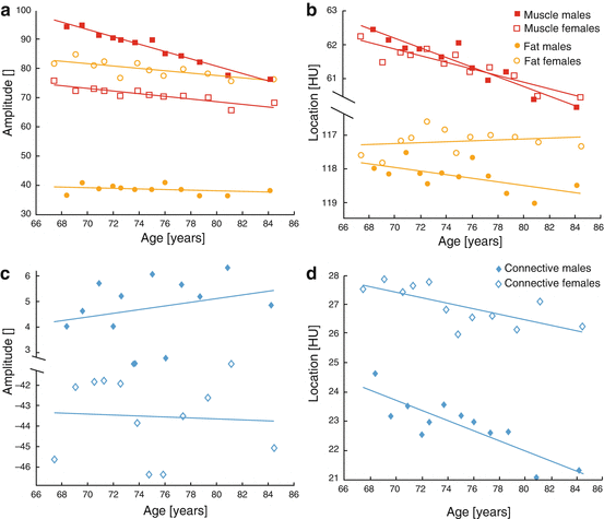
Fig. 24.2

HU distribution profiling results for over 3000 healthy elderly subjects. Linear regression was performed for (a) muscle and fat amplitudes, (b) muscle and fat locations, (c) connective tissue amplitudes, and (d) connective tissue locations

Figure 24.2 illustrates clear differences in distribution parameters between men and women, but how these parameters vary and the degree to which they fit to linear correlation with age depends upon the tissue type. The amplitudes of both fat and muscle in both men and women decrease readily with increasing age, but men have significantly higher muscle amplitudes and lower fat amplitudes than women. Intriguingly, the locations of muscle peaks were nearly identical and decreased analogously with age in both men and women, but the women’s fat peak location increased while the men’s decreased. This could be interpreted as evidence that, while both sexes lose soft tissue volume similarly with age, women exhibit increased fat volume and decreased muscle volume compared to men. Furthermore, both sexes’ muscle densities decrease identically with age, suggesting an analogous trend of increased adiposity in both sexes. Increasing densities for fat tissue in women could likewise be a further indicator of fatty tissue infiltration, but this conclusion is less obvious.

The degree of linear correlation in the connective tissue amplitudes and locations was much lower than fat or muscle. However, women and men exhibited marked differences with similar variance in these parameters as a function of age. Connective tissue amplitudes increased with age in men but decreased in women, while the locations decreased analogously with age for both sexes. This could suggest that lower muscle density (increased muscle adiposity) from sarcopenic degeneration could increase predictably with advanced age, but the low linear correlations in these terms give pause for any definitive conclusions.

24.3 3D Modeling: Morphological and Compositional Changes in the Muscle

As previously mentioned, many recent investigations have realized the quantitative potential of CT image analysis to quantify muscle composition and quality, and its utility for analyzing muscle degeneration in particular has been of great focus in research. As such, many investigators have assessed how changes in skeletal muscle density correlate with changes in muscular volume and function in patients suffering from a variety of conditions or diseases. We have already seen the utility of HU distribution analyses in the rigorous quantification of degenerating muscle. However, this section focuses on another utility of these CT-derived density values that has particular relevance in a clinical context: the use of density-based tissue segmentation and 3D modeling to clearly illustrate changes in muscle mass and quality.

Figure 24.3 illustrates how the tibialis anterior muscles of three representative subjects may be reassembled in 3D with voxel coloration that correlates to each of the three tissue types that were defined previously. The compositions of these tissues have likewise been calculated for each leg. As is evident from these values, the elderly subject and pathological subject (who suffered from asymmetrical lower body paralysis from a pelvic mass infiltration of the sciatic nerve) exhibited increasing amounts of fat and loose connective tissue, compared to the control subject. Likewise, the left leg of the pathological subject contains remarkably more fat than the right leg, illustrating the degeneration’s severity.

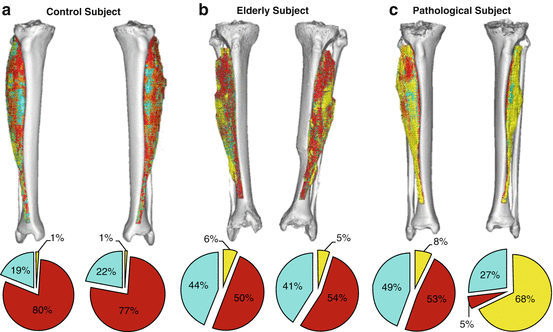
Fig. 24.3

Segmented soft tissues and compositions within the tibialis anterior from each subject’s 3D upper leg volumes. Tissue types are as follows: fat (yellow), connective tissue (cyan), and muscle (red). (a) The control subject’s composition is primarily muscle, but (b) the elderly subject had markedly more fat and connective tissue, to the detriment of muscle. (c) However, the pathological subject’s healthy leg composition was analogous to those of the elderly subject, but the pathological leg comprised of nearly all fat and connective tissue

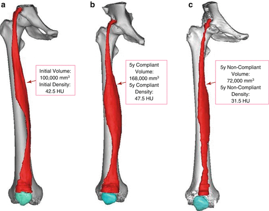
The use of 3D segmentation and modeling can likewise be utilized to show changes in muscle volume and density during a targeted therapy. Figure 24.4 depicts such an example, where a patient with complete lower motor neuron denervation from a spinal cord injury underwent functional electrical stimulation (FES) treatment for 5 years, followed by 5 years of non-compliance to the therapy. It is clear that the increase in both volume and density of the rectus femoris muscle indicates the overall importance of the treatment—which likewise highlights the utility of the 3D segmentation process.