Key points
- 1.
Epidemiology is the study of distribution of disease and factors that determine disease occurrence in populations.
- 2.
As much as possible, medical decisions should be based on quality evidence. The best evidence is a properly designed randomized controlled trial. Evidence from nonrandomized but well-designed control trials is of lesser quality. Next in reliability is well-designed cohort or case-control studies, which have been repeated by several investigators. Opinions of respected authorities and extensive clinical experience are least reliable.
Epidemiology
Epidemiology is the study of distribution of disease and the factors that determine disease occurrence in populations . The focus is on groups rather than the individual . Persons within a population do not have equal risk for disease occurrence, and the risk of a disease is a function of personal characteristics and environmental exposures. Patterns of disease occurrence within specific populations can be evaluated to determine why certain groups develop illness when others do not. The impact of epidemiology on gynecologic oncology is evidenced by the significance of studies such as the association with infection of oncogenic human papillomavirus and cervical cancer, obesity and the risk of endometrial cancer, and the risk factors for gestational trophoblastic neoplasia. Epidemiologic studies are unique in their focus on human populations and their reliance on nonexperimental observations. Epidemiologic methods are used in searching for causes of disease, disease surveillance, determining the cause of disease, diagnostic testing, searching for prognostic factors, and testing new treatments.
Because the quality of epidemiologic evidence varies greatly among studies, the scientific community endorses the principles of Sir Austin Bradford Hill, an eminent British statistician, when attempting to identify causal associations. A cause of a specific disease is an antecedent event or characteristic that is necessary for the occurrence of the disease .
Evidence-based medicine
As much as possible, medical decisions should be based on quality evidence. The best evidence is a properly designed randomized controlled trial. Evidence from nonrandomized but well-designed control trials is of lesser quality. Next in reliability is a well-designed cohort or case-control studies, which have been repeated by several investigators. Opinions of respected authorities and extensive clinical experience are least reliable.
The targets of therapeutic oncology trials have shifted from being predominantly organ specific to being focused on specific patient populations and indications. Clinical trials are more frequently designed to match targeted drugs to the right patient.
Good science depends on accurate (i.e., statistically significant and meaningful) data from clinical trials. The best trials are usually experimental, powered, randomized, and blinded.
Whereas retrospective and observational studies are descriptive and do not involve either an intervention or a manipulation, an experimental study does. A prospective trial poses the question before the data are collected, thus allowing better control of confounding variables, unlike a retrospective study, which poses the question after the data are collected.
Measures in epidemiology
To describe and compare groups in a meaningful manner, it is important to find and enumerate appropriate statistical terms ( Table 21.1 ). Below are concepts integral to the critical review and understanding of the medical literature.
Incidence rate: Measures the new cases of a specific disease that develop during a defined period of time and the approximation of the risk for developing the disease. The incidence rate focuses on events. Incidence measures the probability of developing a disease.
Kappa coefficient: Kappa indicates how much observers agree beyond the level of agreement that could be expected by chance. Kappa is estimated as ( P obs – P chance )/(1 – P chance ). Thus, the kappa coefficient is the observed agreement, corrected for chance as a fraction of the maximum obtainable agreement, also corrected for chance. Landis and Koch have suggested useful categorizations. Kappa = 0.00 should be taken as representing “poor” agreement, 0.00 ± 0.20 as “slight” agreement, 0.21 ± 0.40 as “fair” agreement, 0.41 ± 0.60 as “moderate” agreement, 0.61 ± 0.80 as “substantial” agreement, and 0.81 ± 0.99 as “almost perfect” agreement. A kappa coefficient of 1 represents perfect agreement.
Mean: The average of a sample of observations
Median: The middle value when the values are arranged in order from the smallest to the largest
Meta-analysis: The statistical process of pooling the results from separate studies concerned with the same treatment or issue is frequently used and provides the quantitative backbone of the evidence-based medicine program. Frequently, meta-analyses are undertaken with the broad aim of combining the results of different trials to determine a single estimate of treatment effect. For example, the Cochrane Collaboration endeavors to collate and synthesize high-quality evidence on the effects of important health care interventions for a worldwide, multidisciplinary audience and publishes them in the Cochrane Database of Systematic Reviews. Meta-analyses increase the statistical power by increasing the sample size, resolve uncertainty when reports do not agree, and improve the estimates of effect size. The bias of publication only of positive results is a concern for those using results of meta-analyses because, if statistically significant or “positive” results are more likely to be published, a meta-analysis based on the resulting literature will be biased. The quality of the studies included is important to the quality of the final result.
Study heterogeneity: The statistical measure to assess the excess variation of outcomes contributed by the studies included in the meta-analysis that is beyond that explained by measurement error.
Pearson’s correlation r : The degree to which two variables are related is called correlation. Pearson’s correlation is represented by the value r and varies between −1 and +1. It is usually presented as a scatter point graph. A value of −1 suggests a perfect negative linear relationship, a value of 0 reflects no linear relationship, and a value of 1 reflects a perfect linear relationship. Values of −1, 0, and +1 are rare.
Person time: The sum of the observation period of risk for the persons in a group being studied.
Predictive value positive: The proportion of positive test results that is truly positive (i.e., the probability that someone classified as exposed is truly exposed). This value only refers to positive tests.
Predictive value negative: The proportion of negative test results that is truly negative. The predictive value of a negative test result refers to the proportion of patients with a negative test result who are free of disease.
| Terminology | Mathematical Definition |
|---|---|
| Prevalence rate | Number of persons with disease/Total number in the group |
| Incidence rate | Number of new cases/Total number at risk per unit of time |
| Kappa | ( P obs – P chance )/(1 – P chance ) |
| Sensitivity | True positive/(True positive + False negative) |
| Specificity | True negative/(True negative + False positive) |
| Predictive value positive | True positive/(True positive + False positive) |
| Predictive value negative | True negative/(True negative + False negative) |
These values, unlike sensitivity and specificity, indicate the reliability of the test in the determination of presence or absence of disease.
Prevalence rate: The amount of disease in a population. Prevalence measures the proportion of diseased individuals at a particular time and represents a snapshot of the disease. Other commonly used terms are prevalence proportion and point prevalence . It is a measure of status and includes individuals with newly diagnosed disease and those surviving with disease. The numerator is the number of affected individuals in a specific time period. The denominator is the total number of persons in the group. Prevalence rates range between 0 and 1.
Quality-adjusted life year (QALY): The QALY was developed as an attempt to combine the value length of life and quality of life into a single index number. One year of perfect health is given a value of 1. Death is given a value less than 0. A year of less than perfect health will have a value less than 1. States of health considered worse than death can be argued to have a negative value. The QALY value is determined by multiplying the utility value associated with that state of health by the years lived in that state. QALY is a metric used to compare the benefit of health care interventions. Combination of QALYs with the cost of an intervention (Cost/QALY) can provided an economic framework for comparisons of therapies. QALYs have several limitations and should not be used alone in decision making.
Response Evaluation Criteria in Solid Tumors ( RECIST) : This is a standard for the assessment of response of solid tumors during and after therapeutic interventions for clinical trials.
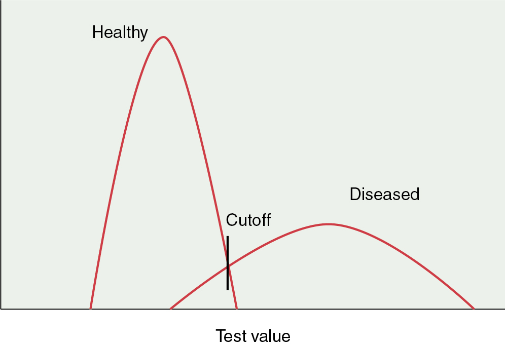
Sensitivity: The proportion of truly diseased persons who are classified as diseased by the test. The sensitivity of a test is therefore the probability of a test being positive when the disease is present. The sensitivity of test may also be called the true-positive rate. In Fig. 21.1 , it is evident that the cutoff point of a test can affect the sensitivity. If the cutoff point is moved to the left, more diseased persons will be identified. At the same time, more healthy persons will be erroneously classified as sick. However, as the cutoff value for normal is moved to the right, the test will become less sensitive because fewer diseased persons will be classified as such.

Figure 21.1
Effects of shifting cutoff point on sensitivity and specificity.
Specificity: The proportion of a population of disease-free individuals who are classified as without disease by a test. In contrast to the sensitivity of a test, the specificity of a test is the probability that a test result will be negative when the disease is absent. The cutoff point of a test for normality influences the specificity. As the value of normality or cutoff moves to the left, the test becomes less specific because fewer healthy individuals are recognized as such. In contrast, moving the cutoff values to the right increases the specificity (see Fig. 21.1 ). In the best scenario, a test would be able to discriminate between diseased and healthy individuals without any overlap. More often, the scenario is as presented in Fig. 21.1 in which there is significant overlap and whatever the cutoff value, healthy persons may be classified as diseased and sick persons classified as healthy . When we set the cutoff point for a test, we must be attentive to the purpose of the test. If the disease is treatable and missing the disease has serious ramifications, then we must favor sensitivity over specificity. Alternatively, if it is more important to correctly identify healthy individuals, then specificity is prioritized. Published reports of the performance of tests usually just provide sensitivity and specificity results. Variations of these measures occur under many conditions and will also produce variations in predictive values.
Standard deviation (SD): A measure of the variability within each group. If there is a normal (bell-shaped curve) distribution, approximately 95% of the values are within 2 SDs on both sides of the average.
Tests of heterogeneity: Before performing a meta-analysis, it is customary to assess evidence of variation in the underlying effects. This variation, termed “heterogeneity,” arises because of differences across studies in populations, exposures or interventions, outcomes, design, or conduct. A forest plot is useful for visual assessment of consistency of results across studies. A statistic that measures the consistency of findings as the proportion of total variation in point estimates attributable to heterogeneity is now widely used.
Analysis of clinical trials
Null hypothesis: This hypothesis, symbolized by H0, is a statement claiming that there is no difference between the experimental and population means. The alternative hypothesis (H1) is the opposite of the null hypothesis. Often in research, we need to be able to test for both the positive and adverse outcomes; therefore, a two-tailed hypothesis is chosen even though the expectation of the experiment is in a particular direction.
Significance level: A level of significance termed the alpha value is determined before the study has begun. The alpha value is the likelihood that a difference as large or larger than that which occurred between the study groups could be determined by chance alone. The alpha level is established by those designing the study and becomes the level of statistical significance. The most typical alpha level is 0.05.
One-tail test: A test to determine a difference in only one direction (e.g., to determine if drug A is better than drug B).
Two-tail test: A test to determine any difference between the variable (e.g., if either drug A or drug B is superior to the other). It is usually considered that in a two-tailed test, more trust can be placed in the statistically significant results than with a one-tailed test. When in doubt, the two-tailed test is preferred.
Confidence interval (CI): This is the method to report the range of uncertainty of a statistically derived estimate. For example, a 95% CI represents the range of values that is believed to contain the true value within a 95% level of certainty.
Alpha error: The rejection of the null hypothesis when it is, in fact, correct; also called a type I error.
Beta error: Failure to reject the null hypothesis when it is, in fact, incorrect; also called a type II error.
Power: The probability that a study will be able to correctly detect a true effect of a specific magnitude. The statistical power refers to the probability of finding a difference when one truly exists or how well the null hypothesis will be rejected. The power is usually specified beforehand in prospective studies. The values of 0.8 (80%) or 0.9 (90%) are typical. The higher the value, the less chance there is of a type II error. A 0.9 value means that a type II error would be avoided 90% of the time. Greater statistical power in a study design will require a larger number of subjects to experience the primary event.
Risk: The proportion of unaffected individuals who, on average, will contract the disease of interest over a specified period of time. Results of a trial are often expressed as absolute or relative risk reductions. The absolute difference is the actual difference between the units of the difference. Relative risk represents the ratio between two percentages. Relative risk reductions often sound much more dramatic than do the absolute values. One must consider the prevalence of a disease when evaluating risk reductions. When there is a low prevalence of a disease process, small risk reductions become unimpressive and must be evaluated in terms of the benefits of a particular mode of therapy.
Incremental cost-effectiveness ratio: The additional cost divided by the incremental benefit compared with an alternate strategy. A strategy was strongly dominated if it was more costly and less effective than another or cost effective if it had an incremental cost-effectiveness ratio of $50,000 to $100,000 per year of life gained relative to an alternate strategy.
Odds ratio (OR): The ratio of the odds that an event will occur in one group compared with the odds that the event will occur in the other group. In an osteoporosis study, if 14 of 22 people who are thin have fractures, the odds of having a fracture are 14 in 22 or 0.64. If 5 of the 33 non-thin people fracture bone, the odds are 5 in 33 or 0.15. The OR is 0.64 divided by 0.15 or 4.2, meaning that thin people are 4.2 times more likely to receive fractures. An OR of 1 means that both groups have a similar likelihood of having an event. Odds ratios are usually linked to statistics derived from logistic regression.
Overall survival (OS): The interval from the completion of treatment to censoring or death from any cause.
Progression-free survival (PFS): The interval from the date of randomization to the documentation of progression of the illness or death from any cause.
Actuarial (life table) survival: This technique uses grouped information to estimate the survival curve. The data are grouped into fixed time periods (e.g., months, years) that include the maximum follow-up. The survival curve is estimated as a continuous curve and gives an estimate of the proportions of a group of patients who will be alive at different times after the initial observation. The group includes patients with incomplete follow-up.
Chi square ( χ 2 ): The primary statistical test used for studying the relationship between variables. This is a test used to compare proportions of categorical variables.
Cox proportional hazard regression analysis: Cox regression analysis is a technique for assessing the association between variables and survival rate. The measure of risk provided for each variable is the risk ratio (RR). An RR of 1 means that the risk is the same for each participant. An RR greater than 1 indicates increased risk; a ratio less than 1 indicates less risk. A ratio of 5.4 means that the patients with a variable are 5.4 times more likely to have the outcome being studied. CIs can also be provided with RRs. This type of analysis is usually presented in a table.
Efficacy: The possibility that an intervention will result in a change (e.g., in vaccine trials).
Imputation: In many analytical scenarios, a case is discarded if it is missing data relevant to the analysis. This may introduce a bias, decrease the power of the study, or alter the representativeness of the results. Imputation is the process of substituting missing data. There are numerous techniques to impute data.
Multivariate analysis: A technique of analysis of data that factors many variables. A mathematical model is constructed that simultaneously determines the effect of one variable while evaluating the effect of other factors that may have an influence on the variable being tested. The two most common algorithms developed to accomplish this task are the step-up and step-down procedures. Variables are added to an initial small set or deleted from an initial large set while testing repeatedly to see which new factor makes a statistical contribution to the overall model.
Propensity score: In studies in which randomization is not possible, investigators use this score to adjust for the bias due to confounding variables inherent in treatment selection for groups being compared (e.g., in observational trials when the treatment of the participants is not random). Assignment to intervention does not occur by chance but depends on patient characteristics that can influence the effect of the intervention on the outcome. The propensity score is the probability that a patient would receive the treatment of interest based on the characteristics of the patient, clinician, and clinical environment. Several different techniques can be used to balance the groups being compared. The most common strategy is propensity score matching. Propensity score methods are usually better than matching on specific characteristics or stratification because it adjusts for confounding better than other strategies. This is a valuable approach when completion of a randomized trial is not feasible.
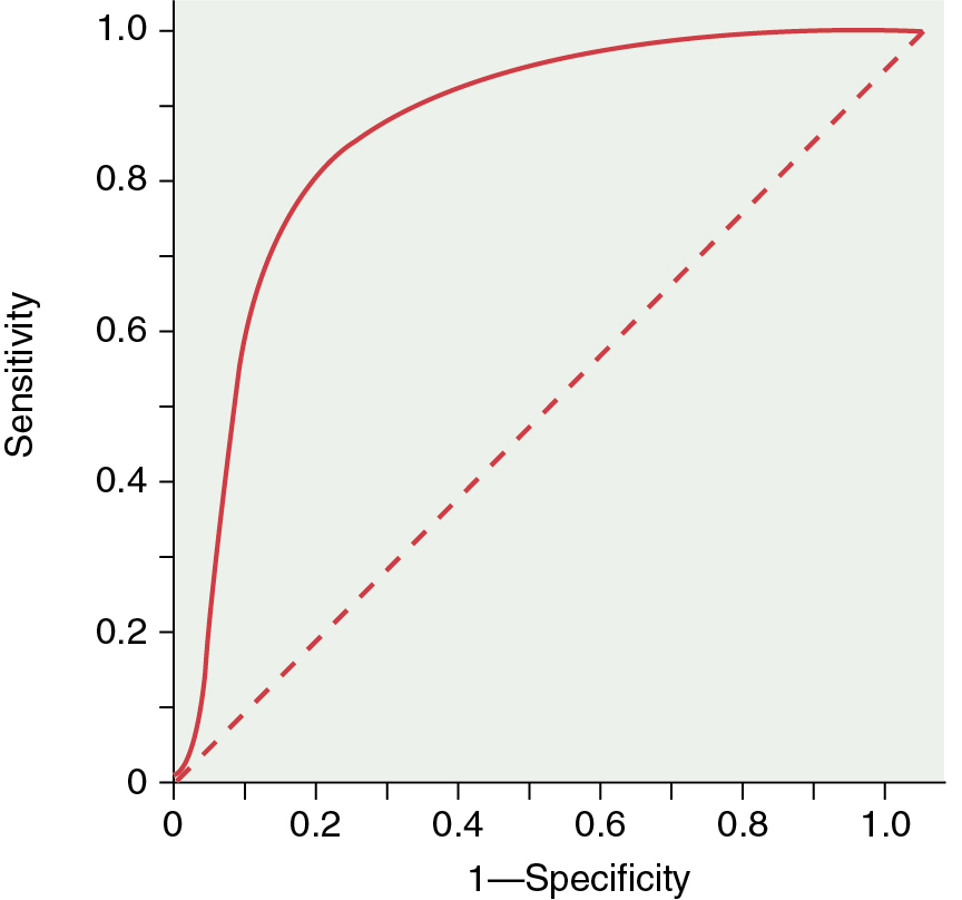
Receiver operator characteristics (ROCs): These curves are the best way to demonstrate the relationships between sensitivity and specificity. The curves plot sensitivity (true-positive rate) against the false-positive rate (1—Specificity) ( Fig. 21.2 ). The closer the curve is to the upper left-hand corner, the more accurate it is because the true-positive rate is closer to 1 and the false-positive rate is closer to 0. Along any ROC curve, one can observe the impact of compromising the true-positive and false-positive rates. As the requirement that a test has a high true-positive rate increases, the false-positive rate will also increase. The closer the curve is to the 45-degree diagonal of the ROC area under the curve, the less accurate the test (see Fig. 21.2 ).


