Treatment Planning Validation

(14.1)

where C _jis the j -th cluster, μ _jis the center of the j -th cluster, and D stands for the distance between the two points. Each data point, x, is a vector described by the eight features (four beam energy values and four monitor units).

To select the number of clusters, we utilized the Bayesian Information Criterion (BIC) as follows [26]:

$BIC\kern0.24em score\kern0.46em =\kern0.46em lnp\left(X\Big|q\right)\kern0.46em -\kern0.46em \frac{M}{2}lnN$

(14.2)

where $p\left(X\Big|q\right)$ is the likelihood of the data $X=\left\{{x}_1,\dots, {x}_N\right\}$ given the model parameters θ, M is the number of free parameters, N is the number of data points, and ln is the natural logarithm. To compute the likelihood, we assumed the followingprobabilistic model: $p\left({x}_i\right)={\displaystyle \sum}_{j=1}^k{\pi}_jp\left({x}_i\Big|\kern0.24em {q}_j\right)$ , with π _jas the proportion of datapoints belonging to cluster j and θ _jas the parameters (mean and covariance) for cluster j. We set the means to be the k centroids in K-means. We estimate the covariance matrix (Σ) of each cluster using the sample covariance matrix of the cluster found by K-means.

$\widehat{S}=\frac{1}{N-1}{\displaystyle \sum}_{x\in {C}_j}\left(x-{\mu}_j\right){\left(x-{\mu}_j\right)}^T$

(14.3)

where T is the matrix transpose operation. For the mixture weights, π _j, we use the relative size of the cluster (the number of data points in the cluster divided by the total number of data points).

The formula for the log-likelihood is provided below:

$L(q)= ln\;p\left(X\Big|q\right)={\displaystyle \sum}_{i=1}^N\ lnp\left({x}_i\right)={\displaystyle \sum}_{i=1}^N ln\;\left({\displaystyle \sum}_{j=1}^K{\pi}_jp\left({x}_i\Big|{q}_j\right)\right)$

(14.4)

The point probability of each data point is calculated as:

$p\left({x}_i\Big|{q}_j\right)=\frac{1}{{\left(2\pi \right)}^{\frac{d}{2}}\left|{\varSigma}_j\right|{}^{\frac{1}{2}}}\kern0.46em {e}^{-\frac{1}{2}{\left({x}_i-{\mu}_j\right)}^T{\varSigma}_j\left({x}_i-{\mu}_j\right)}$

(14.5)

where d is the dimension (number of features) of the data. The number of freeparameters, M, in our model is $\left(k-1\right)+kd+k\frac{d\left(d+1\right)}{2}$ where

is the numberof mixture weights, kd is the number of parameters for the mean vectors, and $k\frac{d\left(d+1\right)}{2}$ is the number of parameters for the covariance matrices.

K-means clustering may be trapped into a local optimum minimum. The quality of the final clustering solution depends on the initial selection of the k cluster centers. To avoid local minima, we used a modified version of PCA-Part [27]. PCA-Part is a deterministic initialization method that has been shown to lead K-means to solutions that are close to optimum. PCA-Part is an initialization algorithm that hierarchically splits the data into two in the direction of the largest eigenvector (first principal axis) at each step until k clusters are obtained. K-means clustering aims to minimize the sum-squared-error criterion. The largest eigenvector with the largest eigenvalue is the direction, which contributes to the largest sum-squared-error. Hence, a good candidate direction to project a cluster for splitting is the direction of the cluster’s largest eigenvector, which is the basis for PCA-Part initialization. Our modified algorithm integrates the K-means clustering algorithm into the PCA-Part initialization algorithm, in order to refine the results at each iteration. This modification helps the partitions converge to final clusters with smaller SSE values.

14.3.2 Outlier Detection

Since there are a large number of patients involved, to avoid statistical bias, we randomly selected 1,000 patients as our training set and used the other 650 patients as testing set. The training set was used to build clusters, while the test set was used to test the model’s outlier detection capability.

We assumed that our training set comprises of normal (“correct”) treatments. We applied K-means clustering to extract similarity groups from these data. In K-means clustering, we assumed that each cluster came from a Gaussian distribution. Since our training data were examples of normal (“correct”) treatment, we tested a new treatment instance as correct or an outlier by testing whether it belongs to any of our Gaussian clusters.

We assigned a rule of classifying a test treatment instance as an outlier if its Euclidean distance from the closest cluster center is greater than a threshold. Because we had a probability distribution model for each cluster, we could set the threshold to assure us of the probability of making a type I error or false positive (i.e., of deciding a point as an outlier when in fact it is normal) is smaller than α. In our experiments, we set the threshold to be 2 sigma (where sigma is the standard deviation), which assures us of the probability of a type I error to be less than 5 %.

For each cluster built based on the training set, we first calculated the mean and standard deviation of all the features (in this study, we have eight features for each treatment plan). To check whether or not a new data point is an outlier, we find a cluster whose center is the closest to the data point using the Euclidean distance and then calculate the difference for each feature between the data point and the cluster center. If the difference is within a preset tolerance (e.g., two standard deviations of that cluster) for all the features, this data point is considered to belong to the cluster. Otherwise, we classified the data point as an outlier.

To measure the quality of the clustering results and how well they could be used to identify outliers, we purposely introduced errors to the test set and used the outlier detection algorithm described above to compute the outlier detection rate. The outlier detection rate is defined as the ratio of the number of data points that are detected as outliers to the total number of data points tested. The outlier detection rates were computed at various error levels for MUs. The error level is defined as the deviation from the original value of an MU feature. For example, 10–20 % error level means that the introduced errors are 10–20 % of the original MU value.

We also introduced errors to the energy features. Unlike the MU features, the possible values of an energy feature are discrete. They can only be one of 6, 10, 18, and 23 MV. Similar to computing the outlier detection rate for MU features, we first randomly selected a patient from the test set and selected a feature out of four energy features (E _AP, E _PA, E _RL, E _LL). We then randomly set the value of the energy feature to one of the three values that are different from the original value. The outlier detection procedure was performed to compute the outlier detection rate for each of the four energy features and for all features combined.

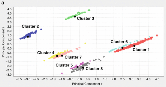
We checked the clustering results by visualizing the data. One way to visualize data in dimensions greater than three is to project it to two dimensions and plot the data in that two-dimensional space. We applied principal component analysis (PCA) to reduce the dimensionality. To be able to visualize the clustering results, we projected the data set onto its first three principal components, as shown in Fig. 14.1a–c. By looking at all the three figures, the separation between the clusters becomes quite clear. For example, from Fig. 14.1a, clusters 4 and 7 projected onto principal components 1 and 2 seem to be very close. However, it does not mean that they are actually one cluster. When we looked from Fig. 14.1b, c, where the data were projected onto principal components 1 and 3 and principal components 2 and 3, respectively, clusters 4 and 7 are clearly separated. That means they are two separated clusters. Similar situations exist for clusters 5 and 8 and clusters 1 and 6. Figure 14.1 also shows that indeed our clustering results (the different colors represent different clusters) make sense, and the cluster means (marked in black dots) are correct.