Treatment Planning Algorithms: Proton Therapy

Hanne M. Kooy

Benjamin M. Clasie

Introduction

A clinical dose computation algorithm, a “dose algorithm,” must satisfy requirements such as clinical accuracy in the patient, computational performance, representations of patient devices and delivery equipment, and specification of the treatment field in terms of equipment input parameters. A dose algorithm has been invariably imbedded within a larger treatment planning system (TPS) whose requirements and behavior often affect the dose algorithm itself. Current clinical emphasis on the patient workflow and advanced delivery technologies such as adaptive radiotherapy will lead to different dose algorithm implementations and deployments depending on the context. For example, a treatment planner needs highly interactive dose computations in a patient to allow rapid evaluation of a clinical treatment plan. A quality assurance physicist, on the other hand, needs an accurate dose algorithm whose requirements could be simplified considering that QA measurements are typically done in simple homogeneous phantoms.

A dose algorithm has two components: a geometry modeler and a physics modeler. In practice, the choice of a physics model drives the specification of the geometry modeler because the geometry modeler must present the physics modeler with local geometry information to model the local effect on the physics-model calculation. Physics models come in two forms: Monte Carlo and phenomenological. The latter models the transport of radiation in medium with analytical forms and has been the standard in the clinic because of the generally higher computational performance compared to Monte Carlo. Monte Carlo, in general, models the trajectories of a large number of individual radiation particles and scores their randomly generated interactions in medium to yield energy deposited in the medium. Monte Carlo is considered an absolute benchmark and much effort is expanded to produce high-performance implementations. The accuracy of a Monte Carlo model is inversely related to the extent and complexity of the modeled interactions and improved performance can be achieved by limiting the model to meet a particular clinical requirement. We describe, as an example, a basic Monte Carlo, which outperforms a phenomenological implementation because of its simple model and implementation on a graphics processor unit (GPU).

The geometry modeler creates a representation of the patient, which is invariably derived from a CT volumetric data set and the CT voxel coordinates are sometimes chosen as the coordinates for the points for which to compute the dose. Dose points are typically associated to individual organ volumes after the dose calculation proper for the computation of, for example, dose-volume histograms. A more general implementation allows the user to select arbitrary point distributions. The geometry modeler also provides the physical characteristics of the patient including, for example, electron density derived from CT Hounsfield Units and, for protons, the stopping power ratio relative to water also derived from CT Hounsfield Units albeit indirectly. The geometry modeler also implements a model of the treatment field. For a Monte Carlo implementation this is a two-step procedure. First, the treatment field geometry and equipment parameters are used to create a representative phase-space, that is, the distribution of particles in terms of position and energy, and perhaps other parameters, of the radiation particles that impinge on the patient. Second, the particles are transported individually through the patient until they are absorbed in or exit the patient volume. For a phenomenological implementation, the treatment field geometry forms a template whose geometric extents are projected through the patient volume. This projection is typically implemented by a ray tracer where individual rays populate the treatment field to sufficiently sample the features within the patient and where the physics model becomes a function of distance along the ray. Figure 10.1 shows the various computational approaches.

Proton transport in medium has been exhaustively studied and the references in this chapter are but a minimum.

Physics of Proton Transport in Medium

Interactions

The physics of proton interactions for clinical energies, that is, between 50 and 350 MeV, is well understood. The publication “Passive Beam Spreading in Proton Radiation Therapy” by Bernard Gottschalk (1) provides an in-depth, theoretical and practical, elaboration of this physics and this section relies significantly on that material.

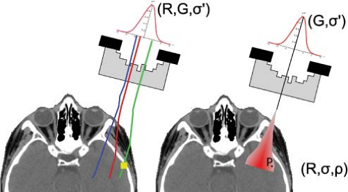Figure 10.1. The left panel shows a Monte Carlo schematic while the right panel shows a phenomenological schematic. The beam includes an aperture and a range-compensator. The beam for both is assumed subdivided in individual pencil-beam “spots.” These spots are physical in the case of pencil-beam scanning (see text) while for a scattered field they are a means for subdividing the field for computational purposes. The initial spot is characterized by a spread σ′, an intensity G and an energy R. In the Monte Carlo, the spot properties can be used as a generator of individual protons. Thus, there will be more “red” protons than “blue” protons than “green” protons. The total number of protons is on the order of 10⁶ or more. Each proton is transported through the patient and its energy loss is scored in individual voxels (a “yellow” one is shown). In the phenomenological model, the spot defines one or more pencil-beams that are traced through the patient. Each ray-trace models the broadening of the protons in the pencil-beam as a continuous function of density ρ along the ray-trace. Dose is scored to points P, where the deposited dose depends on the geometric location of P with respect to the ray-trace axis and the proton range R and pencil-beam spread σ. The latter may include the initial spot spread σ′ if the ray-trace axis represents all the protons G in the spot. Otherwise, the spot can be subdivided into multiple sub-spots such that the superposition of those spots equal the initial spot.

Protons loose energy in medium through interactions with orbital electrons, scatter predominantly through electromagnetic Coulomb interactions with the nuclear electric field, and have inelastic interactions with the nucleus itself. Proton–electron interactions produce delta electrons that deposit dose in proximity to the proton geometric track. The mass of the proton is about 2,000 times that of the electron and hence the collision is equivalent to a blue whale moving at near-relativistic speed toward you: the proton emerges unscattered. Proton–nucleus Coulomb interactions result in small angular deviations in the proton direction and produce, to a very good approximation, a Gaussian diffusion profile in a narrow parallel beam of protons. The Gaussian form of this profile is a consequence of the very large number of random scattering events, which, as described by the central limit theorem, approximate to a continuous Gaussian function to describe the underlying discrete random events.

Protons also have inelastic interactions with the nucleus and produce secondary particles including secondary protons, neutrons, and heavier fragments. The secondary protons contribute up to 10% of the dose within a proton depth dose (2). The secondary neutron production is of specific concern because of their long-range effect. These neutrons deposit dose to healthy tissues throughout the patient, far from the target region, and impact on the shielding requirements of a proton therapy facility. The neutron contribution to the dose distribution is only considered implicitly through their contribution in the physics parameters such as a depth-dose distribution. The effect of heavier secondaries is small and can be ignored for dose calculation purposes.

Relative Biological Effectiveness

Dose deposited by protons is considered to be biologically equivalent to Co60 dose. That is, cellular response to proton and photon interactions are considered equivalent. Clinically, though, the proton physical dose (in Gy) is scaled by an RBE factor of 1.1 to yield the proton biological dose with units of Gy (RBE) (3). Thus, a photon fraction prescription of 1.8 Gy (which implicitly has an RBE of 1 as Co60 is the “standard” dose reference) can be delivered with a proton fraction of 1.8 Gy (RBE), which corresponds to 1.64 Gy physical proton dose. The latter is the value one would measure in a radiation detector and to which one would calibrate the field to deliver 1.8 Gy (RBE).

Clinically, the RBE is assumed 1.1 throughout. Of special consideration is the change in RBE at the distal drop-off of the Bragg peak. In this region, the change in RBE has the effect of differentially shifting the distal edge deeper by about 1 mm compared to measurements. That is, the biological dose fall-off is shifted 1 mm deeper compared to the physical dose fall-off. This inherent uncertainty in the distal edge is one reason why the sharp distal edge is not used to achieve, for example, a dose gradient between a target and a critical structure. The other reason (see below) is the uncertainty in the relative stopping power, which is estimated on the order of 2% to 3%. These uncertainties could result in
overdose to the critical structure or underdose to the target (see Fig. 10.2).

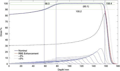Figure 10.2. An SOBP depth dose distribution with its constituent pristine Bragg peak depth dose distributions scaled relative to their contribution. The deepest pristine peak is at 160 mm, which results in a lower SOBP range of 158.4 mm because of the other peak contributions. The 90-90 modulation width is 100.2 mm while the 90-98 is 83.1 mm. The range uncertainties create a band of uncertainty both distally and proximally (see dashed distal fall-offs). The effect is most pronounced at the distal fall-off and the error must be considered to ensure that the target coverage is respected. The 80% depth, R₈₀, of a pristine peak correlates accurately with the proton energy in MeV. The clinical historical range is in reference to the 90% depth which also depends on the energy spread. The difference in practice is on the order of 1 mm. Care should be practiced especially considering calibration and reference conditions.

The RBE, in general, depends on other factors such as dose fraction size, number of fractions, clinical end point, and so on. These factors can be ignored for proton radiation computations but are significant for higher LET charged particles such as Carbon. Computation algorithms for such particles are, therefore, much more complicated and must implement a model for the LET distributions in patient to resolve such dependencies.

Stopping Power

The various electromagnetic interactions transfer energy to electrons in the medium and the proton energy is reduced as a consequence. The proton energy loss, transferred to the medium, is quantified as the rate of energyloss per unit length, d/E/dx, where E (MeV) is the energy and x (cm) is the distance along the proton path. The stopping power S is defined in combination with the local material density ρ (g/cm³):

and is called the mass stopping power.

The mass stopping power in a given medium is a function of the proton energy E and increases significantly when the proton has lost nearly most of its energy. The proton mass stopping power in a given material can be calculated using the Bethe-Bloch equation (4) or directly from tables (5). For example, the mass stopping power values for protons of energies 100, 10, and 1 MeV, respectively in water are 7.3, 45.7, and 261.1 MeV cm²/g. Thus, a proton of 1 MeV energy cannot travel more than 0.004 cm in water. It is this rapid increase in energy loss per unit length, and the very localized energy deposition, that leads to the characteristic Bragg peak of the proton depth-dose distribution (Fig. 10.2). Note that a Bragg peak is a characteristic feature of all charged particles, including electrons, of the energy loss along the particle track. The feature disappears for electrons traversing a medium due to their large scattering angle. In effect, the track becomes “tangled-up” and the Bragg peak becomes averaged out over all the entwined tracks. Thus, a mono-energetic electron depth-dose distribution has a broad and flat high-dose region followed by the distal fall-off.

Water-Equivalent Depth and Proton Range, R

In a photon algorithm, the computational quantity is the radiological path length,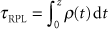

, that gives the density (ρ in units of g/cm³ or relative to water) corrected depth along the ray up to the physical depth z in cm. For a proton algorithm, the appropriate quantity is the water-equivalent thickness, τ_WET in g/cm², which is the thickness in water that produces the same final proton energy as the given thickness in the medium. It is calculated from relative stopping power, S_W^V, defined as the ratio of the stopping power of protons in the medium over that in water. In practice, S_W^V is known for the materials such as polyethylene used in range-compensators or derived empirically from CT numbers (see Fig. 10.3). The proton water-equivalent thickness* along a ray trace is given as

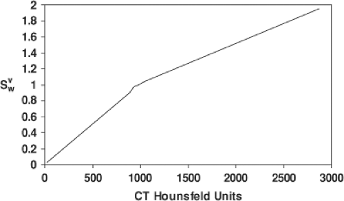Figure 10.3. Conversion from CT Hounsfeld units of the volume to relative stopping power, S_W^V, for biological tissues. Figure is adapted from Schneider et al. [7].

where ρ_w is the density of water.

The mass stopping power ratio,

is almost independent of therapeutic proton energies for biological materials (6). If this ratio is unity, the radiological path length and water-equivalent thickness are mathematically equivalent. In treatment planning, however, the differences between τ_RPL and τ_WET can be clinically significant.

Range, R, which is often called the mean proton range, is the average water-equivalent depth where protons stop in the medium. This is a very close approximation of the range in the continuous slowing down approximation, R_CSDA, and the depth at distal 80% of maximum dose, R₈₀, of a pristine proton Bragg peak (see Fig. 10.2). These definitions of range are often used interchangeably in proton therapy.

Dose to Medium

The dose to a volume element, of thickness t along and area A perpendicular to the proton direction, is given by the energy lost in the voxel divided by the mass of the voxel

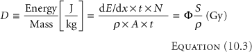
where Φ = N/A is the proton fluence in (cm^-2). Consider a fluence of 10⁹ (1 Gigaproton [Gp]) per cm² of 100 MeV protons in water where S/ρ = 7.3 MeV cm²/g. The dose is (Equation 10.3)

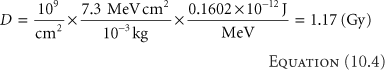
at the entrance of the water (where the proton energy is 100 MeV) and where we used the factor 10^-3 to convert from gram to kilogram and the conversion factor is 0.1602 × 10^-12 J/MeV. Equation 10.4 shows that the number of protons to deliver a clinical dose is on the order of Gigaprotons, a number less than 10^-15 of the number of protons in a gram of water. A convenient rule of thumb is that 1 Gp delivers about 1 cGy to a 1 L (i.e., 10 × 10 × 10 cm³) volume.

The mass stopping power only measures the energy loss from electromagnetic interactions and does not include the energy deposited from secondary particles. In practice, a measured depth dose is a surrogate for the mass stopping power and thus effectively includes all primary and other interactions in calculational models.

A CT data representation of the patient does not provide the necessary stopping power information; it only provides the electron density on a voxel level. The conversion from this electron density to relative stopping power is empirical and is based on an average for particular organs over all patients (7). Thus, the conversion has inherent uncertainties due to (1) the nonspecificity for a particular patient, and (2) the lack of knowledge of precise stopping powers for particular organs. One, therefore, assumes a 3% uncertainty in the relative stopping power in patients (see Fig. 10.2). This 3% uncertainty must be considered by the treatment planner as is described elsewhere.

A dose algorithm may use longitudinal depth-dose distributions in water for all available proton energies. Dose distributions in the patient are calculated from the dose in water using the local density and relative stopping power, both of which come from CT data. In the presence of heterogeneities, the depth-dose distribution in the medium, T_M(E, τ_WET), is obtained from that in water by (following from Equation 10.3 and assuming constant fluence)

where E is the incident proton energy, z is the geometric depth in cm, and the superscript ∞ indicates that broad beam depth-dose distributions are at infinite source-to-axis distance (SAD). The effect of inhomogeneities is twofold. Firstly, the physical depth of the Bragg peak is shifted relative to a water phantom based on the water-equivalent
depth in the patient. The shift for material M with geometric thickness z_M and water-equivalent thickness τ_WET,M is

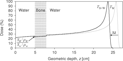Figure 10.4. T_W is the depth dose distribution in a homogenous water phantom and T_W+B is the depth dose distribution in a water phantom with bone at 5 cm depth. The relative mass stopping power,

of bone to water gives the ratio of the dose deposited in bone to water in the shaded region. Bone has larger relative stopping power,

compared to water and, for 2.9 cm geometric thickness of bone with 1.72 relative stopping power, the Δz is -2.1 cm by Equation (10-5b).

Secondly, the dose in the heterogeneity is scaled by the relative mass stopping powers. The latter ratio of relative mass stopping powers is close to 1 and the scaling of the dose is typically ignored in dose algorithm implementations. These effects are illustrated in Figure 10.4.

Only gold members can continue reading. Log In or Register to continue