Treatment Planning Algorithms: Model-Based Photon Dose Calculations
Thomas R. Mackie
Hui Helen Liu
Edwin C. McCullough
Introduction
This chapter takes a different approach to photon dose calculations in radiotherapy. There are several good books and review articles on radiotherapy dose computation algorithms (1,2,3,4,5,6,7,8). In this chapter, we present the current status of computational approaches to predicting radiotherapy dose distributions.
Computational solutions for complex calculations have a predictable evolution. Computer algorithms in the sciences usually begin by mimicking procedures originally designed for hand calculations. Computers made it possible to gather, organize, and synthesize larger volumes of data to provide input for more complex descriptions of the problem. As computers become faster, new opportunities for increased precision or efficiency present themselves. Procedures that would be undreamed of without computers are described algorithmically. For example, computational meteorology began by storing statistical data of weather patterns so that meteorologists could perform their predictions faster. Soon, satellites were providing enormous quantities of data on cloud cover, rainfall, and wind velocity. These data now fuel meteorologic predictions using fluid and heat transport calculations that involve trillions of operations to model or simulate the global weather. Many sectors of the world economy now rely on accurate predictions for agriculture, air and sea transport, and disaster prediction. Radiotherapy treatment planning (RTP) has entered the modeling or simulation phase of computation.
To generate models, it is necessary to understand the system being modeled. In radiotherapy, the system of interest consists of patients and the equipment that delivers their treatments. With the advent of computed tomography (CT) and magnetic resonance imaging (MRI), reliable representations of an individual patient’s anatomy can be obtained at millimeter resolution at reasonable time and cost. Linear accelerators have been routinely used for treating cancer since 1965, but detailed energy spectra about their photon beams were not a high priority. Monte Carlo simulations (MCSs) are routinely used to determine the radiation properties of treatment beams. This information is needed as input data for any model-based treatment planning system. Model-based dose algorithms are used as the basis for the current generation of treatment machines, which will deliver optimized or intensity-modulated radiotherapy (9). Model-based treatment planning demands understanding of the physics of ionizing radiation interactions. Therefore, this chapter provides a short review of the necessary radiologic physics presented in a nontechnical way. Before the background and details of model-based photon dose algorithms can be presented, the history and context of the field must be reviewed.
History of Computation Systems for Radiotherapy
Computerized RTP is more than 40 years old. The first computational techniques applied to radiotherapy are attributed to Tsien (10), who used punched cards to store digitized isodose charts so that the dose distribution from multiple beams could be summed. The dose distribution computed for ∼500 points took approximately 10 to 15 minutes per beam. This was still much quicker than doing this work using tracing paper and a slide rule. The 1960s saw development of batch-processing computer planning systems. The first commercial treatment planning systems were introduced in the late 1960s (11). At the outset, commercial treatment planning systems had the following capabilities:
To store information on the radiation beams used in the clinic
To allow an outline of the patient to be entered
To plan the direction of the beam and the beam outline
To compute the dose distribution
To display the dose distribution with respect to the patient outlines
These features were not very mature in the earliest treatment planning systems. Given the capabilities of the beam and patient representations (e.g., a patient outline), it is not surprising that early dose algorithms were very simple.
The first commercial treatment planning was done on dedicated systems that operated on specialized hardware. The use of dedicated hardware was not isolated to radiotherapy but was the norm for radiology and most small specialized application systems as well. The credit for the use of generic computer systems for radiation treatment planning is attributable to academic institutions. Today, all treatment planning vendors are using generic treatment computer systems controlled by UNIX or Windows-based
operating systems. This development allows treatment planning vendors to take advantage of economies of scale and the latest hardware, but most importantly, it lets them devote more time to software development. In addition, software upgrading, as well as hardware maintenance and longevity, is vastly improved.
operating systems. This development allows treatment planning vendors to take advantage of economies of scale and the latest hardware, but most importantly, it lets them devote more time to software development. In addition, software upgrading, as well as hardware maintenance and longevity, is vastly improved.
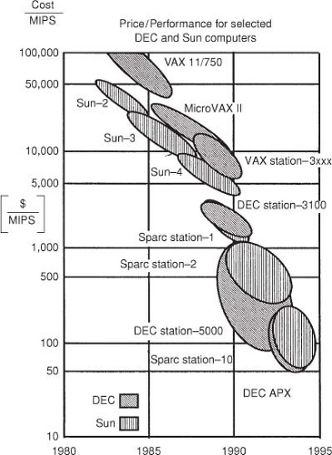 Figure 7.1. A rapid increase in performance is seen if dollars spent per performance (in units of millions of single instructions per second) is plotted for the recent past. The data, which reflect a range of performance characteristics and discounts, are accurate only within a factor of 2. |
Progress in RTP is driven by computer technology. The past 20 years have seen an explosive growth in the capabilities of computers. Figure 7.1 illustrates the price–performance ratio since 1980 in units of dollars spent per million instructions per second (MIPS). In 1980, a VAX computer from Digital Equipment Corporation could cost as much as $1 million and would be able to perform ∼100,000 operations per second. In 2006, a $2,000 computer with an Intel Pentium 4 can perform approximately a billion operations in a second. Similar performance and price improvements have been achieved with other processors. While it is expected that for single-processor systems this growth will slow down during the next decade, multiple (parallel) processor systems are expected to keep the price–performance curve improving. Computer technology has affected RTP in several ways. Faster computers are enabling more advanced computation algorithms to enter into clinical use. Three-dimensional (3D) RTP and the use of more sophisticated algorithms began with the advent of CT, which is required for accurate dose computation. CT and 3D RTP allow more complex beam arrangements, which in turn demands more advanced computation algorithms. Fast image manipulation such as volume rendering, has helped to promote and sell 3D treatment planning systems. These processes require fast computers that can in turn be used for more advanced dose computation algorithms.
There is and will continue to be in the near future a trade-off between accuracy and speed of dose computation. It is important to have a good match between the dose planning algorithms and the computer hardware. Since a great deal of time in modern treatment planning is spent segmenting regions of interest, there is no benefit if the dose computation algorithm is fast and not particularly accurate. Fast but relatively inaccurate algorithms do have a role when many beams must be computed and there is a great deal of iteration on the beam parameters. This occurs, for example, in stereotactic radiosurgery planning. At the opposite extreme, it is counterproductive to have an algorithm that is very accurate but takes an inordinate amount of time to compute. From the point of view of software vendors, it is important to keep software accuracy and speed balanced as the performance of computer systems increases. In many instances, it is useful to have quick calculation models for developing the early stages of a treatment plan.
The Representations of the Patient and the Dose Distribution
Patients have been represented in planning systems in a variety of ways. Hand calculations for monitor unit calculations represented the patient as a block of tissue with a surface normal to the beam at a specified source-to-surface distance (SSD). This representation was highly accurate when the field is rectangular, centered on the central axis, and incident normally on the patient, and when the skin contour is flat out to the extent of the field and the field is in a relatively homogeneous region. A moderate-sized treatment to the abdomen is an example. The simplest patient representations used in RTP systems were one or a few contour lines outlining the skin. These could be acquired in a number of ways, from solder wire surface contours to contours acquired from CT. The contours, entered or digitized into the planning system, represented the skin outline in two or three dimensions. Such procedures resulted in the patient being represented as a homogeneous composition (usually water) but do allow surface corrections to be applied. Patient heterogeneities could be represented in simple ways such as using closed contours like the surface representation. Each inhomogeneity had to be outlined individually, with a density assigned. This could usually be done semiautomatically on CT images for tissue such as lung or bone or for air cavities, where the contrast between tissues was sufficiently high. The electron
density to assign to the region could be inferred from the CT number (12). The problem with this approach was that tissues such as lung and bone are not themselves homogeneous; there is a variation by ∼50% for both bone and lung density. The lung density varies because blood pools from hydrostatic pressure differences.
density to assign to the region could be inferred from the CT number (12). The problem with this approach was that tissues such as lung and bone are not themselves homogeneous; there is a variation by ∼50% for both bone and lung density. The lung density varies because blood pools from hydrostatic pressure differences.
All modern radiotherapy systems use a fully 3D point-by-point or voxel-by-voxel description of the patient. A CT image set of the treatment region constitutes the most accurate representation of the patient applicable for dose computation. This is because there is a fairly reliable one-to-one relationship between CT number and electron density (12) but this correspondence should be established for each kilovoltage energy setting on each CT scanner separately, and this relationship has to be ensured with ongoing calibrations. Dose algorithms that can use the density representation on a point-by-point basis are easier to use because contouring of the heterogeneities is typically not required. An exception to this is when contrast agents can produce a CT number in the bladder or a brain tumor that mimics bone. Usually, the contrast agent is used to aid in the tissue segmentation, and so only the additional step of providing a more realistic CT number in the segmented region is required to correct for the presence of the contrast agent. The spatial reliability of CT scanners is typically within 2% (which corresponds to ±20 in Hounsfield numbers). For photon beams, this uncertainty leads to dose uncertainties of <1% (12). The information in MRI is not strongly related to electron density. An MRI image set can also be more prone to artifacts during image formation. MRI may not replace reliable electron density information for dose computation, and CT will remain the major imaging modality in radiotherapy for the foreseeable future. The use of MRI as an adjuvant to CT will grow, as it is able to provide superior tissue contrast in many cases.
The resolution of the CT voxels and the spacing of the points at which the dose is computed (the dose grid resolution) should be matched. A CT volume set typically consists of 50 to 200 images with resolutions of 512 × 512 × 2 bytes. The voxel is <1 mm in the transverse directions and 1 to 10 mm in the longitudinal direction. The image set requires 25 to 100 MB of storage. The spacing of the dose computation Cartesian grid points for photon beams is typically 1 to 10 mm on each side. Often, the CT slice thickness is chosen as the voxel size of the dose grid. Presently, a fine-resolution dose grid for photon beam calculations has spacing of 256 × 256 × the number of CT slices, so there is more resolution in the CT voxels than in the finest grid used to represent the dose computation. To get acceptable times for image manipulation, the entire CT volume has to be in memory at once. If this is not feasible, it may be appropriate to down-sample the CT image set to 256 × 256. This makes the transverse resolution more closely matched to that of the longitudinal direction and degrades the dose computation little. Degrading the resolution further than 256 × 256, results in unacceptable loss of detail.
There are five options to obtain quicker dose computations as follows:
Use a faster computer
Make the algorithm faster
Make the grid coarser
Restrict the region over which to compute the dose distribution
Allow a nonuniform sample spacing and optimize the points at which to do the calculation
The first solution is the industry standard because of the continually decreasing price–performance ratio. Many of the rest of these solutions have associated problems. As already discussed, making an algorithm faster often means making it less accurate. A coarser grid results in a poorer representation in the high-gradient region. Restricting the dose calculation volume may not be possible if the dose to a large organ has to be computed before a plan figure of merit, such as a dose-volume histogram, is assessed. The last option, while the most difficult to implement, is probably the best choice. The use of a nonuniform sample spacing can significantly speed up the dose computation because the dose does not have to be computed at finely spaced intervals in regions where the gradient is low. Therefore, more computations should be performed in high-gradient regions near beam boundaries.
Basic Radiation Physics for Model-Based Dose Computation
Dose computation in external-beam radiotherapy predicts the dose produced by highly specialized linear-accelerator radiation sources. A basic look at important aspects of megavoltage x-ray production and interaction is required to understand the capabilities and limitations of model-based treatment planning algorithms.
The following are the only radiation physics topics absolutely required to understand treatment planning algorithms:
The production of megavoltage x-rays
The interaction and scattering of photons by the Compton effect
The effects of the transport of charged particles near boundaries and tissue heterogeneities
X-rays produced by fluorescence are unimportant. Interactions through the photoelectric effect do occur in materials with a high atomic number in the head of a linear accelerator, and pair production contributes a few percent to the attenuation of photons at the highest beam energies used, but these processes are far less important than the Compton effect.
Megavoltage Photon Production
Bremsstrahlung, or braking radiation, is produced when electrons interact with the strong Coulomb force produced by a nucleus and to a lesser extent by orbital electrons. The
broad spectrum of photon beams produced by a linear accelerator typically has a peak of 1 to 2 MeV. The mean energy of the beam is roughly one-third of the nominal accelerating energy. Consequently, there is no dramatic change in the characteristics of megavoltage beams with energy. Megavoltage photon beams become somewhat more penetrating with energy, but the difference between a 10- and a 15-MV beam is much less than between a 100- and 150-kV x-ray beam.
broad spectrum of photon beams produced by a linear accelerator typically has a peak of 1 to 2 MeV. The mean energy of the beam is roughly one-third of the nominal accelerating energy. Consequently, there is no dramatic change in the characteristics of megavoltage beams with energy. Megavoltage photon beams become somewhat more penetrating with energy, but the difference between a 10- and a 15-MV beam is much less than between a 100- and 150-kV x-ray beam.
The production of bremsstrahlung occurs when the high-energy electrons produced by the accelerator strike a target, usually consisting of tungsten. The size of the region from which primary photons are produced is one to a few millimeters (13). The finite size of the source results in a small amount of blurring of the edge of the field. The extent of the penumbra also depends on the distance from the collimators to the source.
A primary collimator, fabricated from a tungsten alloy, defines the maximum field diameter that can be used for treatment.
At megavoltage energies, bremsstrahlung is produced mainly in the forward direction. For example, at 10 MV, approximately twice as much photon energy fluence is produced along the central axis as is emitted at approximately 10 degrees from the central axis (14). In a few accelerator models no longer in production, the beam uniformity was obtained by scanning the electron beam before it struck the target. In most C-arm accelerators, to make the beam intensity more uniform, a conical filter positioned in the beam preferentially absorbs the flux along the central axis. In fact, usually the flattening filter slightly overflattens the field so that the intensity increases from the central axis toward the edge of the field. These intensity horns make the dose profile more uniform at depth by compensating for the loss of scatter dose near the edge of the field.
The presence of the field-flattening filter also alters the energy spectrum. The beam passing through the thicker central part of the filter has a higher proportion of high-energy photons and thereby produces a harder beam than does the beam passing through a thinner part of the filter closer to the field edge. Treatment units that are dedicated to IMRT, for example, the Hi-Art™ (TomoTherapy Inc., Madison, WI) helical tomotherapy system, do not have a field-flattening filter because if a uniform field is needed it can be modulated flat (15).
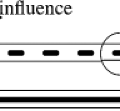
Figure 7.2 illustrates the production of bremsstrahlung photons in a target of a clinical linear accelerator and filtering the beam with a field-flattening filter.
Compton Scatter
Compton scatter influences several aspects of treatment planning with computed dosimetry. There are two general sources of scatter: the treatment head and the patient (or phantom). Production of scatter from either source depends in a complex way on the size and shape of the field. Scatter deep within the patient is mostly generated in the patient. However, at shallower depths and for higher-energy beams the accelerator-produced scatter contribution can be somewhat higher. Much of the complexity of computation-based treatment planning is due to quantifying the magnitude and spatial distributions of these sources of scatter.
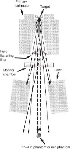 Figure 7.2. The treatment head of a clinical linear accelerator. Primary photons, produced in the target, are shown by the continuous lines. Scattered photons produced in the primary collimator, field-flattening filter, and collimator jaws are shown by dashed lines. These scattered photons have a relatively higher contribution to the photon fluence just outside the field. They are also responsible for the increase in the head-generated output factor as the collimator jaws are opened up. |
While the primary x-ray beam can be thought of as being emitted at a finite source position, it is subsequently contaminated by electrons and photons scattered (extrafocal radiation) within the head (Fig. 7.2). This has been shown experimentally by several investigators (16,17,18,19). The primary collimator and the field-flattening filter produce most of the scatter dose generated by the accelerator head. The primary collimator is close to the target and defines the maximum field radius. More photons interact in this component than in any other in an accelerator, but the vast majority do not escape it. Those that scatter out of the primary collimator do so close to the target and therefore at small radial distances from the central axis. The field-flattening filter intercepts a large fraction of the
photons incident on it, mostly by Compton scattering. The photons produced by the accelerator head must be mainly forward-directed to escape the accelerator. The energy spectrum of the accelerator-generated scattered photons overlaps with the primary beam’s energy spectrum to a large extent (i.e., has nearly the same penetration characteristics as the primary beam), so the difference must be accounted for only quantitatively, not qualitatively. As the collimator jaws open, more scattered radiation is allowed to leave the treatment head. In addition, increasing the jaw opening decreases by a small amount the number of photons backscattered from the jaws into the monitor chamber. This causes the feedback circuit to increase the accelerator current. Both of these effects are reflected as an increase in the machine-generated output with field size, which is traditionally measured in air with a miniphantom (Fig. 7.2). This has been called collimator scatter (5). Even though the collimator jaws themselves contribute little forward scatter, they act as apertures for scatter produced higher in the treatment head. The photons scattered in the primary collimator and field-flattening filter also add to the photon fluence just outside the geometrical field boundary. Helical tomotherapy produces less proportion of scattered photons directed at the patient because of an absence of a field-flattening filter and because the scatter produced by the primary collimator tends to be trapped in downstream collimation.
photons incident on it, mostly by Compton scattering. The photons produced by the accelerator head must be mainly forward-directed to escape the accelerator. The energy spectrum of the accelerator-generated scattered photons overlaps with the primary beam’s energy spectrum to a large extent (i.e., has nearly the same penetration characteristics as the primary beam), so the difference must be accounted for only quantitatively, not qualitatively. As the collimator jaws open, more scattered radiation is allowed to leave the treatment head. In addition, increasing the jaw opening decreases by a small amount the number of photons backscattered from the jaws into the monitor chamber. This causes the feedback circuit to increase the accelerator current. Both of these effects are reflected as an increase in the machine-generated output with field size, which is traditionally measured in air with a miniphantom (Fig. 7.2). This has been called collimator scatter (5). Even though the collimator jaws themselves contribute little forward scatter, they act as apertures for scatter produced higher in the treatment head. The photons scattered in the primary collimator and field-flattening filter also add to the photon fluence just outside the geometrical field boundary. Helical tomotherapy produces less proportion of scattered photons directed at the patient because of an absence of a field-flattening filter and because the scatter produced by the primary collimator tends to be trapped in downstream collimation.
Scattered photons produced in the patient, while directed mainly forward, contribute to dose in all directions. Like scatter produced by the machine, phantom scatter increases with the size of the field. However, for phantom-generated scatter, the penetration characteristics of the beam are also altered. As the field size increases, the phantom scatter causes the beam to be significantly more penetrating with depth. This effect is significant enough that dose computations, using measured dose distributions directly, must tabulate the penetration characteristics as a function of field size.
The behavior of scatter from beam modifiers such as wedges intermediate between the accelerator head and the patient can mimic the effects of either machine-generated or phantom-generated scatter. When the beam is small, a beam modifier mainly alters the transmission and does not contribute much scatter that arrives at the patient. A multiplicative correction factor (e.g., the wedge factor) that includes both attenuation and the small amount of scatter simply and effectively describes the altered dosimetric properties. However, when the field is large, beam modifiers begin to alter the penetration characteristics of the beam, much as phantom scatter does. For example, the increase in the wedge factor with increasing field size and depth is because of beam characteristics altered largely by scatter from the wedge (20,21).
Electron Transport
Photons are indirectly ionizing radiation. The dose is deposited by charged particles (electrons and positrons) set in motion from the site of the photon interaction. At megavoltage energies, the range of charged particles can be several centimeters. The charged particles are mainly set in forward motion but are scattered considerably as they slow down and come to rest. The indirect nature of dose deposition results in several features in photon dose distributions.
The dose from an external photon beam builds up from the skin of the patient because of the increased number of charged particles being set in motion distal to the patient’s surface. This results in a low skin dose, which spares the patient significant radiation injury. The dose builds up to a maximum at a depth, dmax, characteristic of the photon beam energy. At a point in the patient with a depth equal to the penetration distance of charged particles (which is somewhat greater than dmax), charged particles coming to rest are being replenished by charged particles set in motion, and charged particle equilibrium (CPE) is said to be reached. (Later, a distinction will be made between CPE and transient charged particle equilibrium [TCPE] that includes consideration for the reduction in the photon fluence with depth.) In this case, the dose at a point is proportional to the energy fluence of photons at the same point. The main criterion for CPE is that the energy fluence of photons must be constant out to the range of electrons set in motion in all directions. This does not occur in general in heterogeneous media, near the beam boundary, or for intensity-modulated beams.
Electrons produced in the head of the accelerator and in air intervening between the accelerator and the patient may be called contamination electrons. The interaction of these electrons in and just beyond the buildup region contributes significantly to the dose, especially if the field is large. Figure 7.3 illustrates contamination electron depth–ionization curves for a variety of megavoltage photon beams obtained by magnetically sweeping electrons out of the photon field (22). When the depth axis is normalized to the depth at which the contamination falls to 50% of its maximum value, the curves are nearly energy independent.
CPE does not exist near the field penumbra. In fact, for most linear accelerators most of the field penumbra is due to the fall of equilibrium as electrons that leave the field are not replenished from outside the field. CPE is established only at points farther from the field boundary than the lateral range of electrons.
Perturbation in electron transport can be exaggerated near heterogeneities. For example, the range of electrons is three to five times as long in lung as in water, and so beam boundaries passing through lung have much larger penumbral regions. Bone is the only tissue with an atomic composition significantly different from that of water. This can lead to perturbations in dose of only a few percent (23), and so perturbations in electron scattering or stopping power are rarely taken into account. Bone can therefore be treated as “high-density water.”
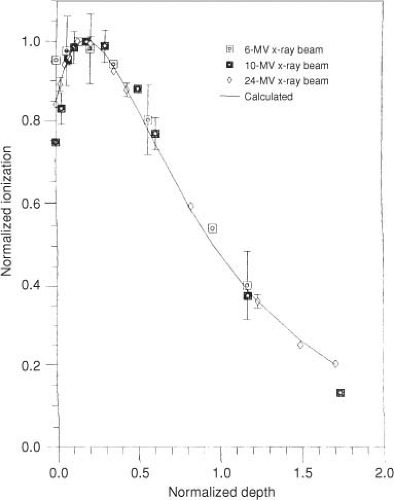 Figure 7.3. The contamination electron ionization as a function of normalized depth in an acrylic phantom. The line is a best fit of data from 6-, 10-, and 24-MV photon beams using the following equation: where I(X) is the normalized ionization curve and X is the normalized depth defined by X = d/d50. The d50 values in acrylic for the electron contamination components from 6-, 10-, and 24-MV photon beams are 0.89, 1.74, and 2.44 cm, respectively. To scale these d50 values to water, multiply by 1.11. (Reprinted from Jursinic PA, Mackie TR. Characteristics of secondary electrons produced by 6-, 10-, and 24-MV x-ray beams. Phys Med Biol 1996;41:1499–1509, with permission.) |
Algorithms for Dose Computation
Traditionally, a patient dose distribution was based on correcting dose measurements obtained in a water phantom. Several types of corrections are applied as follows:
Corrections for beam modifiers, such as wedges, blocks (irregular fields), and compensators, which take into account that a typical field is not the measured open field (i.e., without modifiers)
Contour corrections, which take into account the irregular surface of the patient as opposed to the flat surface of a water phantom
Heterogeneity corrections, which take into account that the patient consists of heterogeneous tissue densities instead of a homogeneous tank of water
The magnitude of the correction is much different for each type of correction. Beam modifier corrections are the most important. For example, 60 degrees beam wedges may result in the fluence under the heel (thick end) of the wedge to be a factor of 3 to 5 less than under the toe of the wedge. Beam intensity in intensity-modulated radiotherapy may vary by a factor of 10. Heterogeneity corrections can result in -10% to +30% change in the dose distal to lung, depending on the size of the field and the lung thickness (24). Under conventional coplanar radiotherapy, contour corrections were the least important, especially if missing tissue compensators were used. Often, these compensators were designed on the basis of missing tissue only, and the errors in this inherent assumption were rarely >3% (25). However, contour corrections are more important than inhomogeneity corrections for relatively homogeneous treatment regions such as the abdomen.
Related posts:

Stay updated, free articles. Join our Telegram channel

Full access? Get Clinical Tree


