Treatment Planning Algorithms: Electron Beams
Faiz M. Khan
Most commercial treatment planning systems incorporate electron beam planning programs. However, not all programs have comparable accuracy or limitations. In general, the electron beam algorithms are more complex than those of the photon beams and require more careful testing and commissioning for clinical use.
Early methods of computing dose distribution were based on empiric data or functions that used ray line geometries assuming broad-beam depth dose distribution in homogeneous media. Inhomogeneity corrections were determined with transmission data measured with large slabs of heterogeneities. These earlier methods have been reviewed by Sternick (1).
The major problem with the use of broad-beam distributions and slab geometries is that this approach is inadequate in predicting the effects of narrow beams, sudden changes in surface contours, small inhomogeneities, oblique beam incidence, and so on.
An improvement over the empiric methods came about with the development of algorithms based on age-diffusion equation by Kawachi (2) and others in the late 1970s. These models have been reviewed by Andreo (3). A semiempiric pencil beam model developed by Ayyangar and Suntharalingam (4) and based on age-diffusion equation was adopted for the Theraplan treatment planning system (Theratronics, Kanata, Ontario). This semiempiric algorithm, if properly implemented for a given electron accelerator, allows reasonably accurate calculation of dose distribution in a homogeneous medium. Contour irregularity and inhomogeneities are considered only in the plane of calculation, as for example, a computed tomography (CT) slice, without regard to the effects of the third dimension, such as adjacent CT slices. Although pencil beams placed along the surface contour can predict effects of contour irregularity and beam obliquity, inhomogeneity corrections are still based on effective path length between the virtual source and the point of calculations. In these cases, bulk density of the inhomogeneity in the given CT slices is used to determine effective depth. The main limitation of such algorithms is that the effects of the anatomy in three dimensions are not fully accounted for, although empirically derived correction factors may be used in simple geometric situations (5).
Pencil Beam Models Based on Multiple Scattering Theory
In the early 1980s, there was a significant surge in the development of electron beam treatment planning algorithms (6,7,8,9). These models were based on Gaussian pencil beam distributions obtained with the application of Fermi–Eyges multiple scattering theory (10). For a review of these algorithms, see Brahme (11) and Hogstrom (12).
Pencil beam algorithms based on multiple scattering theory are the algorithms of choice for electron beam treatment planning. A brief discussion of these algorithms is presented here to familiarize the users of these programs with the basic theory involved.
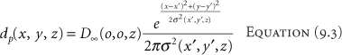
Assuming small-angle approximation for multiple scattering of electrons, the spatial distribution of electron fluence or dose from an elementary pencil beam penetrating a scattering medium is very nearly Gaussian at all depths. Large-angle scattering events could cause deviations from a pure Gaussian distribution, but their overall effect is considered to be small. The spatial dose distribution for the Gaussian pencil beam can be represented thus:
where dp(r,z) is the depth dose contributed by the pencil beam at a point at a radial distance r from its central axis and depth z, dp(o,z) is the axial dose, and σr2(z) is the mean square radial displacement of electrons as a result of multiple Coulomb scattering. It can be shown that σr2 = 2σx2 = 2σy2, where σx2 and σy2 are the mean square lateral displacements projected into the X, Z and Y, Z planes. The exponential function in Equation 9.1 represents the off-axis ratio for the pencil beam, normalized to unity at r = o.
This is another useful form of Equation 9.1.
where D∞(o,z) is the dose at depth z in an infinitely broad field with the same incident fluence at the surface as the pencil beam. The Gaussian distribution function in Equation 9.2 is normalized so that the area integral of this function over a transverse plane at depth z is unity.
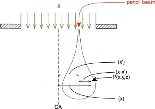 Figure 9.1. A pencil beam coordinate system. Dose at point P is calculated by integrating contributions from individual pencil beams. |
In Cartesian coordinates, Equation 9.2 can be written thus:
where dp(x,y,z) is the dose contributed to point (x, y, z) from a pencil beam whose central axis passes through (x′, y′, z) (Fig. 9.1).
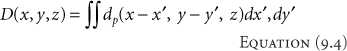
The total dose distribution in a field of any shape can be calculated by summing all the pencil beams:
The integration of a Gaussian function within finite limits cannot be performed analytically. To evaluate it, this function necessitates use of the error function. Thus, convolution calculus shows that for an electron beam of a rectangular cross section (2a × 2b), the spatial dose distribution is given thus:
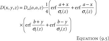
where the error function is defined thus:
The error function is normalized so that erf(∞) = 1. (It is known that the integral 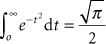 .) Error function values for o < x < ∞ can be obtained from tables published in mathematic handbooks (13). Although, D∞(o, o, z) in Equation 9.5 is given by the area integral of the dose from pencil beams over an infinite transverse plane at depth z, this term is usually determined from measured central axis depth dose data of a broad electron field (e.g., 20 × 20 cm). .) Error function values for o < x < ∞ can be obtained from tables published in mathematic handbooks (13). Although, D∞(o, o, z) in Equation 9.5 is given by the area integral of the dose from pencil beams over an infinite transverse plane at depth z, this term is usually determined from measured central axis depth dose data of a broad electron field (e.g., 20 × 20 cm). |
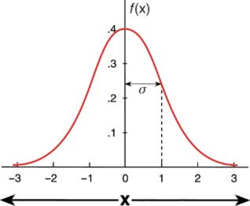 Figure 9.2. Plot of a normal distribution function given by Equation 9.7 for σ = 1. The function is normalized to unity for limits -∞ < x < +∞. |
Pencil Beam Characterization
Lateral Spread σ
As discussed earlier, the spatial dose distribution of an elementary pencil electron beam can be represented by a Gaussian function. This function is characterized by its lateral spread parameter σ, which is similar to the standard deviation parameter of the familiar normal frequency distribution function:
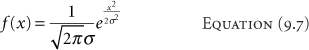
Figure 9.2 is a plot of the normal distribution function given by Equation 9.7 for σ = 1. The function is normalized so that its integral between the limits -∞ < x < +∞ is unity.
As a pencil electron beam is incident on a uniform phantom, its isodose distribution looks like a teardrop or onion (Fig. 9.3). The lateral spread (or σ) increases with depth until a maximum spread is achieved. Beyond this depth there is a precipitous loss of electrons as their large lateral excursion causes them to run out of energy.
The lateral spread parameter σ was theoretically predicted by Eyges (10), who extended the small-angle multiple scattering theory of Fermi to the slab geometry of any composition. Considering σx(z) in the X–Z plane,
Related posts:

Stay updated, free articles. Join our Telegram channel

Full access? Get Clinical Tree


