Treatment Planning Algorithms: Brachytherapy
Kenneth J. Weeks
Introduction
Brachytherapy involves the treatment of cancer using the photon, electron, and positron emissions from radioisotopes. Brachytherapy was developed using naturally occurring radioisotopes such as radium 226. The history, applications, and emission details of radioisotopes are described in Chapter 17 and elsewhere (1,2,3,4). It is the goal of brachytherapy treatment planning to determine how many sources, their individual strengths, and the location of each source relative to the treatment volume, so as to treat a volume to a given minimum dose while respecting tolerances of normal tissues. It is important to note that the original brachytherapy clinical applications were developed realizing that brachytherapy demanded three-dimensional (3D) planning because the sources were distributed in three dimensions. Because of this fact and the absence of computers, these original treatment systems were all inclusive. They were systems with rules for distributing the sources, rules for picking and arranging source strengths, and given the latter, precalculated dose-rate tables for determining the dose to a point. The Manchester, Paris, Stockholm, Memorial, and Quimby systems (1,2,3,4) all specified in alternate ways how to do this for interstitial and intracavitary implants. See Chapter 17 for discussion of these systems. From this history, we can obtain knowledge of the range of the radioactive source applications, which is important in devising dose calculation algorithms. Thus, we summarize guidelines, which include the following. When distributing lines of sources, attempt to keep them spaced no closer than 8 mm (smaller volumes) and no farther than 2 cm (larger volumes) apart. The periphery of the treatment volume is generally not much farther than 5 cm from the center of gravity of the source distribution. The very high doses close (<5 mm) to the sources are not prescribed or evaluated as to clinical significance. At distances >10 cm from the center of the implant, the dose delivered is low and the precise dose is not considered a treatment objective. Therefore, we conclude that dose calculation algorithms that are very accurate from 5 mm to 5 cm and generally accurate to 10 cm are required. The availability of computers and advanced imaging capabilities means that precalculated dose tables for predetermined patterns of multiple sources are no longer required. Calculation of the dose distribution for the individual patient’s source distribution is possible.
Radioisotopes decay randomly with a time-independent probability (1,3,5,6). If there are N0 radioactive atoms at time t = 0, then at a later time t, we have N(t) atoms given by
where λ (= 0.693/T1/2) is the radioisotope’s decay constant and T1/2 is the half-life (time it takes for half of the sample to decay). The activity (A) at time t is proportional to the number of radioactive atoms present and is defined by
where A0 is the initial activity. Throughout the following, we will consider the calculation of the dose rate, [D with dot above] (in cGy/h). The total dose D delivered during an implant, which lasts for time t, is found from the initial dose rate, [D with dot above]0, at the start of the implant from
For the case t ≫ T1/2 (e.g., a permanent implant), the total dose (D) is simply D = 1.44 T1/2[D with dot above]0, whereas if t ≪ T1/2, then D = t[D with dot above]0. Throughout the following, we will calculate the dose rate at the start of the implant ([D with dot above]). The total dose delivered in time t is then found from Equation 8.3.
The isotope emits energy (in the form of photons, electrons, and sometimes positrons) in all directions and that energy is absorbed in the mass (tissue) around the isotope, giving rise to absorbed dose (absorbed energy/mass). The calculation of dose rate depends on the number of radioactive atoms, the types and energies of the emitted particles, the time rate of emission of those particles, and finally the energy absorption and scattering properties of the surrounding media and the radioactive material itself. In this chapter, we will begin with the simplest case of a point source. From there we will use the point source result to determine the dose rate for an ideal line source and then a real clinical cylindrical source. Finally, we will obtain the dose rate distribution for a 3D source/shield/applicator via numerical integration of the point source result. Various intermediate parameterized calculation methods are discussed. This leads inevitably to systems, which explicitly
model the flow of energy from the radioactive sources. These include Monte Carlo and Boltzmann transport theory. These latter techniques owe their existence to the extensive computation power now available. The advantages and disadvantages of these methods will be discussed.
model the flow of energy from the radioactive sources. These include Monte Carlo and Boltzmann transport theory. These latter techniques owe their existence to the extensive computation power now available. The advantages and disadvantages of these methods will be discussed.
Calculation of Dose Rates Around a Point Source
A point source is the simplest situation to calculate. The first approximation, used in radiation oncology, is to ignore the charged particle emissions and consider only the photons. The significance of this approximation is best understood by reviewing the basic nuclear decay data (7). Consider the well-known 192Ir, which has a half-life of 73.8 days and decays via β decay (95%) or electron capture (5%). The decay of a single 192Ir nucleus produces on average 2.38 photons (there are 44 possible photon energies ranging from 7.8 to 1,378 keV, which can be emitted in a single decay event) and 0.95 β-decay electrons (with the β decay continuous energy spectrum ranging from 0 to 669 keV). In addition, atomic electrons can be emitted with various discrete energies ranging from 11 to 1,378 keV. In a single decay, the average total energy output from photons is 813 keV (note the average energy of the photons is therefore 341 keV from 813 keV/2.38) and the average electron energy output is 216 keV (7). Therefore, the total average energy output per decay is 1,029 keV. Our decision to ignore the emitted electrons means that we are going to ignore around 21% of the total energy output from the source in our dose-rate calculations. Why is this justified? The reason is that practical commercial sources used for radiation oncology will be encapsulated radionuclides and that encapsulation will scatter and slow down the electrons such that most do not leave the source capsule itself and for those that do escape, their range in tissue outside the source is much smaller than 5 mm and thus will not contribute dose at a clinical prescription distance. This encapsulation of the source is essential for the clinical use of most isotopes used in radiation oncology. Historically, in the early days of radiotherapy, in the United States, a clever technique to enclose radon gas in glass capsules was developed. The high energy of the β particles and the light filtration led to unfavorable clinical results (4). We end this discussion with the observation that there can be a major clinical dose distribution difference between an encapsulated and an insufficiently encapsulated radionuclide.
Consider a sample of radioactive material whose largest dimension is much smaller than 0.1 mm. This will be small enough so that all atoms can be approximately considered as located at a single point. Restricting ourselves to the photon emissions from the point source, we will first think about the dose rate produced in a small volume (dV) of tissue located at a distance (r) from the source. For simplicity, consider the source in vacuum (so no scatter) and that in each decay it emits exactly one photon with energy E. The situation is shown in Figure 8.1. The dose rate must be equal to the product of the following: time rate of emission of the photons (i.e., activity A), the probability of the photon hitting dV (we will abbreviate that as P[r, dV]), the probability that the photon of energy E, which hits dV actually interacts with dV as opposed to just passing through (P[E, dV]), and the average amount of energy (dEabs) that is absorbed in dV whenever a photon interacts with it, all divided by the mass (m) of dV. The units are energy/mass/time, which is dose rate. Explicitly,
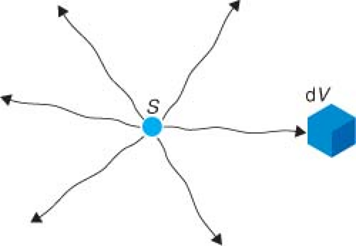 Figure 8.1. Point source (S) emission of photons (wavy lines) in vacuum. Direction is random. Only the photon emitted straight at dV can deposit energy in dV and then only if it randomly interacts with the material in dV. |
The first question is, what happens to the dose rate in dV if we simply change its distance from r to R (Fig. 8.2)? The two things that do not change, at all, are the activity of the source and the mass of the tissue that we move around. P(E, dV) and dEabs should not change if the angles with which the photons hit the volume are similar, that is, the solid angle subtended by dV is small. So, we are left to focus on the probability of a photon hitting dV. When a nucleus decays and gives off a photon, that photon is emitted isotropically, which means the photon is equally likely to go in any direction. Let the cross-sectional entrance area of the mass m be denoted as da (Fig. 8.2). Of course, the total surface area at a distance r is 4πr2. So, the probability
of a photon emitted in a random direction hitting da after it has traveled a distance r is
of a photon emitted in a random direction hitting da after it has traveled a distance r is
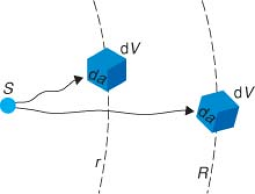 Figure 8.2. Point source (S) emission of photon radiation in vacuum. Cross-sectional area (da) of small material volume dV faces the source. dV is moved from radius r to radius R, causing a reduced probability of being hit by the photons by the factor r2/R2. |
If we move to a larger distance R, the probability of hitting da now equals da/(4πR2). Therefore, the probability of hitting da has been reduced by a factor of r2/R2 in moving from r to R. This suggests that we can try and approximate Equation 8.4 simply as
where we have defined that c = P(E, dV)dEabs/m and we are hoping that c is a constant, under the assumption that the factors in c do not change much as we move the small volume around in vacuum.
In Equation 8.6 it is understood that we should not move the little volume of tissue someplace where it makes no sense to assume that c remains constant. A counterexample best illustrates why it is not true that c is a constant. Suppose that we had moved the volume dV and centered it on r = 0, so that it completely surrounded the radioisotope. The factor P(r, dV), where we got r2 from the first place, is now P(r = 0, dV) = 1, that is, every photon emitted from the radioisotope hits the volume. One can easily see from Equation 8.4 that the dose rate does not become infinite at r = 0 (as Equation 8.6 implies). In fact, depending on the photon energy (E) and the size of dV, the dose rate (from the photons emitted) could be extremely small. This example clearly shows the algorithms we devise to calculate dose rate have their regions of validity.
Historically, radioisotope emissions were first measured in air. In particular, the concept of exposure (1,3,6 and Chapter 17) (amount of ionization of air per unit mass) was used extensively because charge collection in air-filled cavities are the easiest measurements to make. The process was, first, measurement of exposure rate in air, second, conversion of that exposure rate in air to dose rate to a small amount of tissue in air, and finally, conversion to dose rate to a point in the patient. The result of this process (1,3) led one to define a dose rate to a small amount of water at a distance r surrounded by air as
where the single constant c in Equation 8.6 is split into two constants. Γ is the exposure rate constant (in units of R cm2/mCi/h), which represented the conversion of photon energy to ionization of air for the given isotope and fmed (in units of cGy/R) is the conversion constant from exposure in air to dose to medium (water) at the average photon energy given off by the radioisotope. Normally, people choose to express dose to water since its radiation properties are similar to tissue and measurements were/are made in water. Values of f and Γ are given in Tables 17.1 and 17.3 for various radionuclides. The interested reader should refer to Chapter 17 for a further discussion of each quantity.
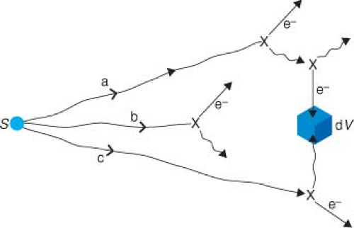 Figure 8.3. Point source (S) emission of photon radiation in homogeneous water medium. Wavy lines are photons, straight lines are electrons, and cross (x) marks are photon interaction points. Three photons are followed. Photon a: Compton scatters above dV, the electron produced misses dV, and the Compton photon scatters again (just above dV). The Compton electron after slowing down deposits its remaining energy in dV. Photon b: It was aimed right at dV coming out of S but halfway it was scattered. Both the Compton photon and electron miss dV. Photon c: Compton scatters below dV and the scattered photon heads right for dV and is photoelectrically captured inside dV; its photoelectron (not shown) is absorbed in dV. |
In Equation 8.7, we have the dose rate to water in air, but what we ultimately want is the dose rate in water (i.e., to the patient). Let us look again at a source radiating photons towards dV but this time in a full water medium. Figure 8.3 shows three examples of photon histories. First, a photon that was going to miss dV (“a” in Fig. 8.3) is scattered several times. Eventually, a secondarily scattered electron deposits a fraction of the original energy into dV. Second, a photon (b), which is emitted from the source aimed right at dV interacts on the way there and no part of its energy reaches dV. Finally, a photon (c), which was going to miss dV, interacts and the scattered photon from that interaction is completely absorbed in dV.
One thing we might guess is that inverse square is not going to be valid anymore because how dV absorbs energy is much more complicated. However, we remember that, inverse square was not a law anyway, and what we want is an approximation in a restricted region of interest. In any event, we could start by describing the dose rate to a point r in water as
In this equation, the major effect of attenuation is represented in the first term where we exponentially attenuate the in-air dose rate of Equation 8.7 with the linear attenuation coefficient (μ) of water for the average energy E emitted by the radionuclide (Table 17.6 for typical values). The exponential attenuation factor takes care of one of these effects above (photon [b] in Fig. 8.3) and scatter out of the path from the radionuclide to dV. Dscat now represents the result
of all the various scatter possibilities and is far more complicated. Equation 8.8 has merely organized the calculation into a primary part and a secondary scatter part. Now, we note in Figure 8.3 that the attenuation scattering events (b) reduce the dose rate in dV but the scatter events (a and c) increase the dose rate relative to the (Fig. 8.1) in-vacuum case. Maybe, if we get lucky, these will cancel out. It turns out that scatter and attenuation effects do not cancel out at all distances from the source, but close to the source they almost do and their change with distance farther away can be simply parameterized. Meisberger et al. (8) showed that the measured variation in dose rate in water as r changed from 1 to 10 cm was such as to establish Equations 8.9 and 8.10 as a good approximation for the dose rate to water
of all the various scatter possibilities and is far more complicated. Equation 8.8 has merely organized the calculation into a primary part and a secondary scatter part. Now, we note in Figure 8.3 that the attenuation scattering events (b) reduce the dose rate in dV but the scatter events (a and c) increase the dose rate relative to the (Fig. 8.1) in-vacuum case. Maybe, if we get lucky, these will cancel out. It turns out that scatter and attenuation effects do not cancel out at all distances from the source, but close to the source they almost do and their change with distance farther away can be simply parameterized. Meisberger et al. (8) showed that the measured variation in dose rate in water as r changed from 1 to 10 cm was such as to establish Equations 8.9 and 8.10 as a good approximation for the dose rate to water
Application of this algorithm (Equation 8.9) has, in the past, been a popular choice in commercial computerized treatment-planning systems. Technically, fmed should now be a function of r to account for the lower energy of the scattered photons with greater distance in water (9,10); however, that detail is usually ignored. Comparing the in-air Equation 8.7 with the in-phantom Equation 8.9, the difference is simply the inclusion of the parameterized factor T(r). T(r), the attenuation and build-up factor, is a polynomial in r (Equation 8.10), which Meisberger et al. (8) used to represent the ratio of the exposure in water to the exposure in air. The free parameters A, B, C, D are determined by least squares fit to the experimental data for each isotope. One sees in Table 17.6 that the value for A is close to 1.0 and that the other coefficients are small. Because of this, the value of T(r) is very close to 1.0 up to a certain distance. Attenuation and in-scatter are balanced at a distance rA where T(rA) = 1.0. That in-scatter cancels out the attenuation loss was pointed out by Hale (11), and is not obvious. For instance, if we consider 137Cs (E = 662 keV), that distance is around 3 cm. If we estimate the reduction in dose from attenuation of 3 cm of water (by using the value for μ in Table 17.6), we would expect a 23% drop-off. Clinically, the fact that a simple dose calculation such as in Equation 8.9 can be used, instead of something as in Equation 8.8, makes calculations easy both by hand and by early computers, and has been extremely useful. The mathematical form, Equation 8.10, which was chosen by Meisberger et al. (8) for T(r) is not a unique parameterization of the attenuation and scatter effects. One could with equal ease use the form proposed by Evans (12)
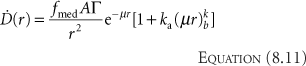
Kornelson and Young (13) fit the coefficients ka and kb to Monte Carlo results (14). Venselaar et al. (15) extended the range of the fitted data to 60 cm. The values for various isotopes are given in Table 17.6. Other mathematical expressions (16,17,18) have also been utilized; there is little difference of clinical significance between them or Equations 8.9 and 8.11. The reader should note that Equation 8.9 or 8.11 can be used with the values in Tables 17.1, 17.3, and 17.6 to perform quick hand-check verifications of clinical implant plans. If one looks at a dose rate at a point 10 cm from the implant center, all the implanted sources can be considered approximately as one point source located at the center of gravity of the implant. Add all the activities together and calculate the cGy/h value expected and compare it to your treatment planning system isodose line. One cannot use this method to determine a small error in the computer plan result, but one can use it to uncover the presence of a major error.
Comparing Equations 8.8 and 8.11, the first term is identical and is the attenuated primary in-air dose rate. Comparing the second terms, one can see that Equation 8.11 assumes that [D with dot above]scat is proportional to the attenuated primary dose rate. This is physically reasonable since scatter comes from the attenuation that occurs in the out-of-path directions and this should be similar to the in-path attenuation. To the extent that this is not true, we make up for that by letting ka and kb be completely free parameters for each different isotope. Fitting the parameters can be done in two ways: one is fitting the free parameters to match measured data and the other is fitting (13,14,15) to match a better calculation such as Monte Carlo. All the parameters (A, B, C, D, and ki) have no direct physical meaning. They are chosen to allow us to describe the dose rate as accurately as possible. Because of that, it is required to keep track over what range of data the parameters were determined. For example, the best-fit value of D just happens to be negative (Table 17.6) for 192Ir, 198Au, and 137Cs. Hence, at large distances (r > 25 cm), where the term r3 in Equation 8.10 dominates T(r), (T(r) = 25 cm) is negative, and therefore Equation 8.9 predicts negative dose rate for those isotopes at large distances. This negative dose result arises because we have applied Equation 8.9 outside the range of the fitted parameters and have obtained a nonphysical (wrong) result.
Calculation of Dose Rates Around a Line Source
In Equation 8.9, we now have an expression for the dose rate in water due to a simple point source. We can now apply this result (we could have just as easily used Equation 8.11 instead) to help us calculate the dose rate from different source geometries. The next simplest case is a line (length L) of radioactive material (Fig. 8.4). In the point source case, we had spherical symmetry, which meant that the direction from the source did not change the dose, only the distance (r) did. With a line source we need to consider direction and distance relative to the center of the line. There is still symmetry remaining, specifically rotational
and reflection symmetry, so if we can calculate the dose rate to every point in the shaded region, the dose rate anywhere else in the patient volume is determined. For example, the dose rate at P in Figure 8.4 is the same as at point B (reflection of P with respect to Y–Z plane), C (reflection of P with respect to X–Y plane), or D (reflection of B with respect to X–Y plane). Moreover, any point off the plane (y ≠ 0) of Figure 8.4 that can be mapped to a point in the plane of Figure 8.4 by a rotation about the z-axis will have the same dose rate as that point in the plane.
and reflection symmetry, so if we can calculate the dose rate to every point in the shaded region, the dose rate anywhere else in the patient volume is determined. For example, the dose rate at P in Figure 8.4 is the same as at point B (reflection of P with respect to Y–Z plane), C (reflection of P with respect to X–Y plane), or D (reflection of B with respect to X–Y plane). Moreover, any point off the plane (y ≠ 0) of Figure 8.4 that can be mapped to a point in the plane of Figure 8.4 by a rotation about the z-axis will have the same dose rate as that point in the plane.
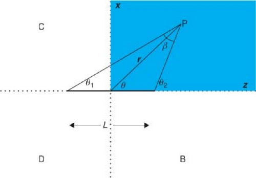 Figure 8.4. Line source geometry. Dose-rate calculation to point P depends on distance and direction (r, θ) of P from the source center. The active length (L) defines angles (θ1 and θ2) from the endpoints of the line source to point P. β = θ2 – θ1 is the angle from P to the endpoints of the active source. Results need to be calculated only for the shaded quadrant; dose to points B, C, and D will be identical to point P by symmetry, likewise for all points in 3D space obtained by rotation of the source about the z-axis. |
The solution can be found in an analytic form by defining an activity per unit length (A/L) of source and integrating the point source expression of Equation 8.9 along the line of the source (dl) to obtain the dose rate at any point P(r, θ) in the plane (19). The final result is
where L is the active length of source and β = θ2 – θ1 is the angle subtended by the line source when viewed from point P.
Calculation of Dose Rates Around an Encapsulated Cylindrical Source
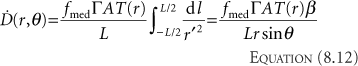
Most applications in radiation oncology entail the use of encapsulated (e.g., stainless steel) cylindrical sources. Consider a cylindrical source S (radioactive source radius rS, active length L) and enclose it (Fig. 8.5) inside a cylinder of encapsulation material (radial wall thickness t and end cap thickness te). Again, we will consider the active source region to be divided into many small point sources and determine the contribution from each point source separately using Equation 8.9 and add the results. Clearly, the first-order effect of the encapsulation will be to reduce the dose rate by an amount that depends on the path lengths through the encapsulation. As the path length through the encapsulation from every small point source to a given dose point is different, the reduction will be different in different directions. The solution to an encapsulated line source was given by Sievert (20). He presented the equivalent (T(r) was ignored in those days) of the following expression for the dose rate at a point P located at planar coordinates r and θ (measured from the radioactive source center, Fig. 8.5)
 Figure 8.5. Cylindrical encapsulated source geometry, thickness of encapsulation is t, radius of source is rS, and the end cap thickness is te. Radioactive material in the source region is subdivided into N tiny regions. Photons from each of these regions are attenuated by their path length through source material and encapsulation. Dose rate at P (located at r, θ from center of source) involves repeated application of point source calculation for all N cubes. For the ith cube, its distance to P is ri, the path through the source material is dSi, and through the encapsulation is dei. |
where μe is the attenuation coefficient for the radioisotope’s photons through the encapsulation material, t is the perpendicular wall thickness of the encapsulation, and θ1 and θ2 are the angles from the point P to the ends of the active length of the source. The integral expression in Equation 8.13 is the Sievert integral, which can be numerically evaluated with a computer. Young and Batho (21) later provided expressions for an effective wall thickness accounting for source radius. As an aside, Γ would be the unfiltered exposure rate constant (1,3,5,6) in Equation 8.13 because the attenuation of the source’s photons by encapsulation is explicitly calculated. The differences between filtered and unfiltered (6,22,23) exposure rate constants are discussed in detail in Chapter 17.
Equation 8.13 is valid for points (such as P in Fig. 8.5) in the patient where path lengths do not go through the ends of the source. Expressions (19,20) that give the dose
rate in the other geometrically distinct regions (through ends of the source capsule) will not be presented here, as calculations involving numerical integration (21) can be obtained with computers. We can present a single equation for calculation anywhere in the region by numerical integration. We subdivide the source volume into N equal parts. Each little source volume element i contributes independently to the dose rate at P. The dose rate at a point P located at r, θ, from the center of the source is given by adding all N exponentially attenuated point source contributions
rate in the other geometrically distinct regions (through ends of the source capsule) will not be presented here, as calculations involving numerical integration (21) can be obtained with computers. We can present a single equation for calculation anywhere in the region by numerical integration. We subdivide the source volume into N equal parts. Each little source volume element i contributes independently to the dose rate at P. The dose rate at a point P located at r, θ, from the center of the source is given by adding all N exponentially attenuated point source contributions
Related posts:

Stay updated, free articles. Join our Telegram channel

Full access? Get Clinical Tree


