10 Three-Dimensional Conformal Radiotherapy and Intensity-Modulated Radiotherapy

Ping Xia, PhD, Lei Xing, PhD, Howard I. Amols, PhD, C. Clifton Ling, PhD

The success of radiotherapy depends on the radiosensitivity of the particular tumor being treated relative to that of the surrounding normal tissues. The goal in radiotherapy, therefore, is to sufficiently separate the dose-response curves of local tumor control and normal tissue complications. During the past decade, advances in radiologic imaging and computer technology have significantly enhanced our ability to achieve this goal through the development of three-dimensional (3-D) image-based conformal radiotherapy (CRT) and intensity-modulated radiotherapy (IMRT). The implementation of these technologies permits better shaping of the high-dose volume of the radiation treatment so as to better conform to the tumor volume while minimizing the radiation dose delivered to surrounding normal tissue. Success of 3D-CRT and IMRT critically relies on the accurate delineation of the tumor volume, augmented with multiple imaging modalities such as the magnetic resonance imaging (MRI), positron emission computed tomography (PET/CT), and four-dimensional computed tomography (4D-CT). Organ motion, change of the patient’s anatomy, and the tumor response to radiotherapy call for the transition from 3D-CRT to 4D-CRT.

IMRT is becoming a mature technology, and is widely applied to many cancer sites. Many treatment-planning comparison studies have demonstrated the clear dosimetric advantages of IMRT.¹^–⁶ Clinical results from the past decade have shown the improvement of local tumor control and reduction of treatment toxicities for prostate cancer, head and neck cancer, and other types of cancer.⁷^–¹⁴

In this chapter, we describe the rationale and processes for 3D-CRT and IMRT, including patient imaging and simulation, treatment planning, dose calculation algorithms, plan evaluation, treatment verification, treatment delivery, and quality assurance (QA) issues. In this discussion, we identify the similarities and differences between 3D-CRT and IMRT, and emphasize those features and benefits unique to IMRT.

Three-Dimensional Conformal Radiotherapy and Intensity-Modulated Radiotherapy Treatment Planning Process

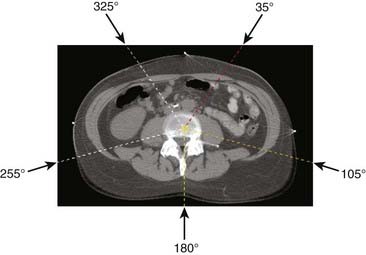
Conventional radiotherapy entails irradiation of the patient from a few beam directions (as the accelerator rotates about the patient), using beam configurations such as that shown in Fig. 10-1, which depicts a five-field isocentric treatment of the prostate. Usually all beams are aimed at a single point denoted as the isocenter that geometrically represents the intersection of the axis of rotation of the linear accelerator gantry head, the collimator assembly, and the treatment couch. Although most often the geometric center of the tumor is purposely positioned at the isocenter, 3D-CRT and IMRT planning do not stringently require that the isocenter be located at the geometric center of the tumor. In many special clinical scenarios (such as in treatment plans for head and neck and breast cancer), the isocenter may be deliberately placed on a specific location, off the geometric center of the tumor. Even though the intervening superficial tissues receive higher radiation doses than does the tumor for each individual beam, the summation of all beams results in a higher dose to the tumor. With conventional radiotherapy, the radiation shape (or aperture) from each beam is manually drawn on the projected two-dimensional (2-D) images, taken from an x-ray machine (referred to as a simulator), which simulates the geometry of a treatment machine (a linear accelerator). With easy access to computed tomography (CT) in modern radiotherapy departments, planning CTs are acquired for most patients undergoing radiotherapy. Sometimes the CT unit, equipped with a flat couch top and alignment laser system, is referred to as a CT simulator. After acquiring a planning CT, the treatment tumor volumes are directly delineated on the CT images, and the radiation portals (or apertures) are designed to conform to the tumor volumes. The difference between conventional radiotherapy and 3D-CRT lies in whether the planning CT is used to define tumor volume and to design treatment portals accordingly. Therefore, 3D-CRT entails more sophisticated shaping of the dose distribution than does conventional radiotherapy because the collimation design (or shaping of fields) and the selection of beam directions are based on 3-D CT images of the patient. These images, projected in a so-called beam’s eye view (BEV) format (described more fully later), permit us to select beam directions with short pathways to the tumor and better avoidance of normal tissues. IMRT goes one step beyond 3D-CRT by enabling variations of the radiation intensity within each beam. This intensity modulation can be achieved via several different approaches, including fabrication of complex physical compensators (often fabricated with computer-controlled milling machines) to be placed in the radiation beam between the radiation source and the patient, but more commonly via the use of a multileaf collimator (MLC) capable of dynamic beam delivery or use of multiple static beams sequentially altered in shape by the MLC. The details of these delivery methods are discussed in the third section of this chapter, “Delivery of Intensity-Modulated Treatment.”

FIGURE 10-1 • Five-photon beams aim at the isocenter for treatment of prostate cancer.

First, let us briefly describe the process of 3D-CRT and IMRT, after which we present details of each step in the process. The treatment planning steps for IMRT and 3D-CRT are similar during the initial and final steps, but diverge in the middle. In particular, patient imaging and simulation are identical for both processes. IMRT differs from 3D-CRT in some of the key steps of plan optimization, which we will discuss along the way. The treatment planning process begins with “treatment simulation,” which entails setting up the patient on the CT unit (or a CT simulator) in the treatment position. More frequently, patient CT imaging and simulation is being augmented with MRI, PET, and other functional imaging studies to better define the tumor volume and critical sensitive structures.

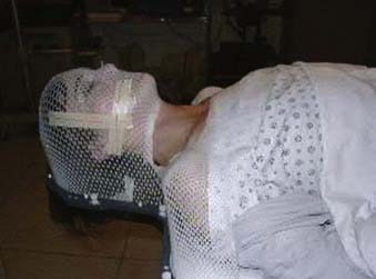
To precisely mimic the patient’s treatment position, simulation first determines a proper posture for the treatment position, including the use of a proper type of immobilization device to facilitate precise reproduction of patient position during simulation, other image acquisition, and multifraction treatment delivery. Often, during the simulation, a patient-specific body mold is fabricated to fix the treatment posture. Fig. 10-2 shows a patient fixed in a head, neck, and shoulder mask on the treatment table. Subsequently, 3-D images are acquired from which the radiation oncologists can delineate target and nearby sensitive structures. Sometimes medical physicists or dosimetrists assist radiation oncologists to contour common sensitive structures, such as the spinal cord, lungs, and liver. The delineation of anatomic volumes is usually done directly on a computer display of transverse CT images using standard computer graphics options such as a mouse, track ball, light pen, and so on. More often, MRI, PET, or PET/CT images are registered with the planning CT to provide better soft tissue contrast (such as in MRI images) and better physiologic information (such as in PET images).

FIGURE 10-2 • A patient is immobilized with a head, neck, and shoulder mask on the treatment table.

Once all relevant tissues have been delineated, the radiation oncologist specifies the desired doses (or the prescription doses) to tumor volumes and the limiting doses to normal tissues. From these specifications the medical physicists or dosimetrists then select and adjust beam directions and design shapes and beam intensities so as to best meet these dose criteria. For 3D-CRT plans, the aperture shape and intensity of each beam is manually designed and iteratively adjusted based on the planner’s experience and intuition. Because the process is performed via “manual” iteration, the quality of the 3D-CRT plan can be constrained by time and by the fact that x-ray beam intensities within each individual beam are uniform (or, if wedges are added, monotonically variable in one dimension only). Once beam directions, shapes, and intensities are specified, the computer calculates the resulting dose distribution, which one compares with the radiation oncologist’s specifications. If there are discrepancies, beam intensities, shapes, and directions are iteratively adjusted (based primarily on the planner’s experience and intuition) and dose distributions recalculated. In practice, only a few parameters can really be adjusted, and each iteration is extremely time consuming. Hence the ability to truly optimize a dose distribution with 3D-CRT techniques is often quite limited. This type of iteration is also referred to as forward planning (FP).

IMRT usually incorporates computerized iteration of radiation beams as opposed to the manual optimization just described. In this process, the computer performs a large number of iterations in less time than a human could perform a few iterations. Further, the computer can modulate the dose intensity within each radiation portal, which is typically divided into multiple pencil beams, each on the order of several square millimeters. The combination of sub-beams of different intensities plus a large number of iterations often enables significantly improved dose distributions with IMRT as opposed to 3D-CRT.¹⁵

Once a treatment plan or dose distribution has been calculated, the radiation oncologist and planner must evaluate the plan to determine how well it meets the original criteria, or dose constraints. This is typically done via analysis of dose distributions and dose-volume histograms (DVHs). When the treatment plan has been accepted for treatment, all of the planning data on beam configurations and radiation intensities are transferred to the linear accelerator (now often done via computer networking systems and “record-and-verify” [R/V] systems) and patient treatment proceeds using the beams designed during treatment planning. For IMRT, the data transferred includes information on dynamic MLC (DMLC) motion files or on static MLC (SMLC) segmental files required to deliver the desired x-ray intensity profiles. Finally, physicists must perform dosimetric and other QA tasks to verify that all equipment is functioning properly, and that the specifics of the dose prescription and treatment plan are accurately delivered to the patient on a daily basis. In the following sections we discuss each of these treatment planning steps in greater detail.

Patient Setup, Immobilization, and Image Acquisition

The minimization of patient set-up uncertainty is more important in 3D-CRT than in conventional radiotherapy because of the improved conformality of the dose distribution (i.e., quick dose gradient between the boundary of tumor volume and normal tissue). This becomes even more critical in IMRT because IMRT plans often produce even sharper dose gradients at the boundary between the tumor volume and normal tissue.¹⁶ Thus, immobilization devices and precise patient positioning procedures must be applied throughout the process of image acquisition, simulation, and treatment. Many different techniques and devices are in use to achieve this, including conventional devices such as vacuum cradles, plaster casts, face masks, and so on. More elaborate devices specific to IMRT are also being introduced such as immobilization devices that attach directly to the treatment couch to ensure that patients are positioned in the same location during each daily treatment. The same “index positioning method” is also used during the CT image acquisition. Stereotactic body frames have also been developed to achieve set-up accuracy approaching that of stereotactic radiosurgery.

In addition to immobilizing the patient, frequent verifications with image guidance are performed to ensure precise reproducibility of the patient position and thus ensure accurate treatment delivery. The first step of image guidance for radiotherapy is to acquire a treatment planning CT, which represents the patient’s body (external anatomy) and internal anatomy. This step is often referred to as CT simulation. CT simulation is performed with a CT scanner with capabilities for spiral or helical scanning and volumetric data acquisition combined with a laser localization system similar to the laser system on the treatment machine such as a linear accelerator, and a high-speed graphic workstation that emulates a treatment planning computer. The laser localization system permits marking the treatment isocenter with fiduciaries on the patient skin, which defines the initial reference point for the entire treatment. It is important that the CT image set is obtained with the patient in the treatment position on a flat couch that is geometrically identical to the couch on which the patient will ultimately be treated. The high-speed workstation provides the capabilities of rapid image reconstruction, target volume and normal tissue delineation, and 3-D beam geometry display. During the CT simulation, the patient’s anatomy is reconstructed from the CT data and displayed in BEV according to the specific treatment set-up parameters. Digitally reconstructed radiographic images provide projected images at a specific view, helping in decision-making and documentation. For moving organs, such as the lungs and liver, new generations of CT scanners with multiple arrays of detectors are capable of acquiring 4D-CT images, providing dynamic views of these moving organs. Digitally reconstructed fluoroscopy from 4D-CT can be displayed as a movie, allowing radiation oncologists to measure the magnitude of the organ or tumor motion in any direction. Furthermore, if the CT images are acquired in synchronization with the breathing cycle, the cine mode of CT images can be constructed into multiple breathing phases, typically eight to ten. To synchronize the CT acquisition with the patient’s breathing cycle, a breathing sensor—either a belt attached to the patient’s chest or an infrared sensor placed on the patient’s chest—is needed.

PET/CT simulation is similar to the CT simulation except the procedure is carried out on a combined PET/CT scanner; again, a flat tabletop and alignment lasers are necessary for the purpose of radiotherapy treatment planning. Direct PET/CT simulation avoids the additional planning CT acquisition, improves the workflow, and reduces the potential errors during image registration if a PET scan is acquired separately or if a PET/CT scan is acquired in a nontreatment position.¹⁷

For some cancer sites (e.g., the prostate), MRI provides much better soft tissue contrast than CT images. MRI simulation can be desirable for reasons similar to the desirability of PET/CT. MRI scanners used in radiology are close scanners, making them inaccessible to the patient once the patient is in the scanner. To set up the patient in a desired treatment position and with a proper immobilization device, an open MRI simulator is preferred. Chen and colleagues ¹⁸ reported their clinical implementation using a 0.23-tesla (T) open MRI scanner for prostate patients. The MRI scanner consists of two poles, which are each approximately 1 meter in diameter. The separation between the two poles is 47 cm. The MRI scanner table can move in and out along a set of rails mounted on the floor and laterally on an orthogonal set of rails built in the couch. Vertical movement of the table is made by using a composite flat top with hard foam spacers beneath the patient. A set of three triangulation lasers (center and laterals) identical to those used on linear accelerators has been used for patient positioning.

The challenge of directly using MRI for radiotherapy treatment planning is that MRI does not contain the electron density information needed for the dose calculation and image distortion in part because of the inhomogeneities in the main magnetic and gradient fields, and in part because of the differentiation in chemical shift and susceptibility of fat and water. With a low magnetic field of less than 0.5 T, Chen and colleagues ¹⁸ report that the latter effect is reduced to 1 to 2 pixels. The distortion caused by the inhomogeneity of the magnetic fields increases as the patient size increases. Even with the distortion correction algorithm, residual distortion was reported greater than 2 cm for lateral patient size larger than 40 cm, whereas the distortion for patient lateral size smaller than 38 cm is insignificant dosimetrically.

Delineation of Treatment Volume and Critical Organs

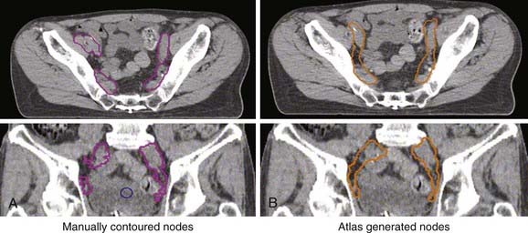
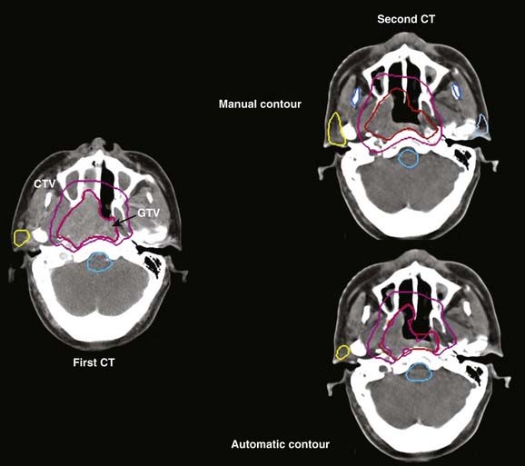
Treatment volumes are defined on the CT images according to International Commission on Radiation Units and Measurements Report 62 nomenclature,¹⁹ with the gross target volume (GTV) defined as the visible tumor as seen on CT or other imaging studies; the clinical target volume (CTV) as the visualized tumor plus regions at risk such as microscopic extension of disease, nodal chains, and so on; and the planning target volume (PTV) as a CTV expanded to include setup errors, patient motion, linear accelerator alignment errors, and other uncertainties. For motion tumor volume, internal tumor volume includes magnitude of movement of the tumor. The manual delineation of CTV, PTV, plus adjacent critical organs is time consuming and subject to large variations among observers. The Radiation Therapy Oncology Group and other groups of experts attempted to establish a consensus to minimize these variations.²⁰^,²¹ Many treatment planning systems now incorporate various software tools for performing automatic delineation of tissue structures, but these are of limited utility as current algorithms are only accurate for outlining external body contours and internal contours of very high contrast such as bone, lung, and air cavities. Other commercial programs and research institutions²²^–²⁶ developed deformable image registration algorithms, permitting the planner to map contours from a template case to a patient case with a similar tumor stage and site but different anatomic characteristics. Fig. 10-3 shows an example of computer-assisted contouring in pelvic lymph nodes. The deformable image registration tools are especially useful when adaptive planning is required for patients with anatomic changes during radiotherapy. Fig. 10-4 shows an example of using deformable image registration to generate contours from an early treatment planning CT (first CT) to the middle-course treatment planning CT (second CT) for a patient with nasopharyngeal cancer while comparing them with manually drawn contours on both CT images.

FIGURE 10-3 • Comparison of the manually drawn (A) and atlas-generated contours (B) of pelvic lymph nodal volumes displayed in an axial image and a coronal image.

FIGURE 10-4 • An example of using deformable image registration to generate contours from an early treatment-planning computed tomography (CT) to the middle-course treatment planning CT for a patient with nasopharyngeal cancer.

Although all of these tools improve the efficiency of laborious contouring and reduce differences in observations among practitioners, it is expected that human intervention will likely remain a necessary and important component for defining tumor volumes, especially the GTV. These tools can significantly improve consistency and efficiency of sensitive structures.

It should be emphasized that in IMRT, accurate delineation of the tumor volume and critical organs is even more important than in 3D-CRT because with inverse planning (IP) optimization the delineated contours are used as direct input to the computer optimization algorithm (as discussed later), which attempts to produce dose distributions conforming to the prescribed dose constraints of the delineated tumor and sensitive normal structures. For similar reasons, it is often necessary with IMRT and inverse treatment planning to contour many normal tissues in the vicinity of the PTV that would not normally be contoured for 3D-CRT treatment planning. This is necessary in order to “advise” the optimization algorithm as to where it is permissible and impermissible to deposit moderate or high doses. For example, in a typical head and neck case, in addition to the commonly contoured structures in 3D-CRT planning such as the spinal cord and brainstem, it may also be necessary to contour the parotid glands, optic structures, the oral cavity, the mandible, the inner ears, and so on, lest the optimization algorithms unwittingly deposit large doses to these volumes to meet dose constraints placed on other structures.

Selection of Treatment Beams

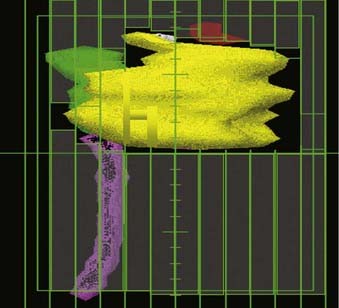
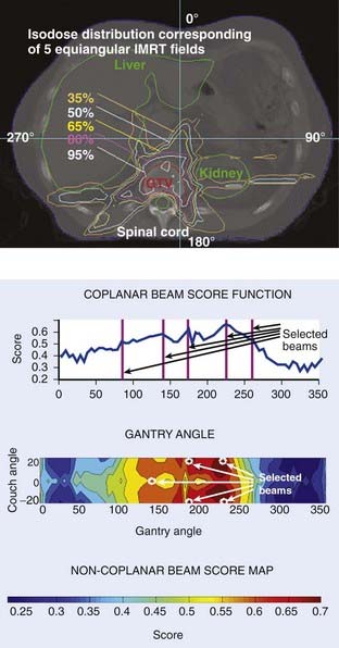
To facilitate selection of beam angles and field shapes based on the relative positions of various anatomic structures, various display schema have been developed for 3D-CRT to represent the PTV and the adjacent critical organs in 3-D perspective on a 2-D computer display monitor. The treatment geometry is usually best visualized in BEV when the anatomy is viewed from the perspective of the radiation source,²⁷^,²⁸ as shown in Fig. 10-5. Beam orientations are chosen by observing the patient in BEV from various beam directions and selecting those directions for which the PTV appears to be best separated from the normal tissues. The BEV, however, considers only the geometric property of the patient. The concept has been extended to BEV dosimetrics (BEVDs), in which both anatomy and dosimetric tolerances of the target and involved organs are taken into account for guiding the beam-placement process. BEVD objectively evaluates the goodness of angular space, and it has shown that the incorporation of the BEVD score in IMRT planning can greatly facilitate the selection of beam configuration.²⁹^–³³ In Fig. 10-6, we show the score functions for an IMRT treatment of a paraspinal tumor obtained with and without BEVD guidance.²⁹

FIGURE 10-5 • The beam’s eye view of a right-anterior oblique angle for a head-neck patient in a supine position with the beam shape as defined by a multileaf collimator (MLC). The planning target volume (PTV) is depicted in yellow, the brainstem in green, the spinal cord in purple, and the pituitary gland in red. Note how the MLC leaves (transparent green) are shaped to conform to the PTV.

FIGURE 10-6 • Isodose distributions of an intensity-modulated radiation therapy treatment with five equiangular beams (40°, 110°, 180°, 255°, 325°). The middle and bottom plots show the beam’s eye view score for the patient for coplanar and non-coplanar beam configurations, respectively.

(From Pugachev A, et al: Role of beam orientation optimization in intensity-modulated radiation therapy, Int J Radiat Oncol Biol Phys 50[2]:551–560, 2001.)

Clinically, selection of beams is based on a combination of experience, standard protocols, and patient-specific anatomy. For example, the relatively small variations from patient to patient in the anatomic relationship between the prostate and its nearby critical structures (most importantly the rectum, bladder, and urethra) enables IMRT prostate treatment plans to follow a more or less standard protocol with regard to beam selection. A treatment planning template can be developed for each specific cancer site.³³^,³⁴ For brain tumors, on the other hand, beam selection is depends on the patient-specific anatomy and the experience of the individual planner. In general, IMRT fields with large fluctuations in intensity require higher velocities and accelerations of MLC leaves during beam delivery. Selection of optimum beam directions is often more critical when treating PTVs with a complex shape or where there is minimal separation between the PTV and a critical normal structure. Carefully selecting optimum beam directions in IMRT may also reduce the complexity of intensity profiles (i.e., the magnitude of intensity gradients within the field), thus improving delivery accuracy and efficiency. Automation of beam configuration selection is still an active area of research. Unfortunately, at present, none of the available IMRT treatment planning systems can effectively determine optimum beam directions, and thus still rely on the treatment planner’s experience and intuition.

Treatment Planning

Forward Planning

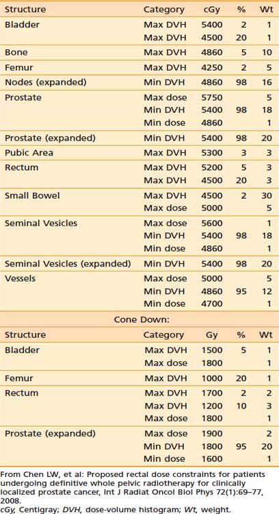
In contrast to IP (discussed in the following section), forward treatment planning involves the planner manually selecting the number of beams, their directions and shapes, inclusion or exclusion of hard or dynamic wedges (wedges modulate beam intensity monotonically along a selected direction), and the relative weightings of each beam shape (the static beam intensities). The computer simply calculates the resultant dose distributions from these beam parameters. In the sense of FP, the dose distribution is predictable by the beam parameters set by the planners. This is fundamentally different than IP in which the human treatment planner specifies the desired dose constraints (ideally, the desired dose shapes or distributions) and the computer calculates the required beam intensities and shapes to best meet the specified dose constraints. The specified dose constraints are a simplified description of dose shapes or distributions because it is not intuitive to depict a desired dose distribution. Table 10-1 provides an example of the desired dose constraints of a concurrent treatment of the pelvic lymph nodes and prostate cancer plus a cone down to the prostate alone.

Table 10-1 An Example of the Desired Dose Constraints of a Concurrent Treatment of the Pelvic Lymph Nodes and Prostate Cancer Plus a Cone Down to the Prostate Alone

In either case, after the computer calculates the resultant dose distribution, the planner may choose to make adjustments to improve the plan. In FP, the planner adjusts the beam intensities (or weights) and may adjust the field shapes or directions, and then asks the computer to recalculate the dose distribution. This process, referred to as manual optimization, is repeated until an optimal dose distribution is obtained. The experience of the individual planner is critical in FP. Even for a skilled planner, the quality of the plan may be limited by the restricted number of degrees of freedom one has, particularly the constraint that intensity within each field must be uniform. Further, the number of iterations one can perform within the allotted time is clearly limited. For IP, the philosophy behind plan optimization is completely reversed.

The advantage of FP is in its ability to produce a simple plan with a small dose variation inside the tumor volume.³⁵^,³⁶ For example, in a treatment plan of a breast, Mayo and colleauges³⁷ compared 3D-CRT plans with wedges to FP-IMRT, IP-IMRT, and a hybrid of open fields and some IP fields. This study reported that the tangent-only IMRT plans, created with an IP method, resulted in the worst dose homogeneity inside the breast, the worst maximum dose outside the target, and 2.3 times more monitor units (MUs) than the FP-IMRT plans. In combining two open tangents with tangent IMRT beams,³⁷ it was found that a plan quality comparable to FP-IMRT could be achieved in significantly less planning time.

Inverse Planning

Principle of Inverse Planning

Inverse treatment planning was first proposed by Brahme in 1988.³⁸ With this process, the user does not directly attempt to optimize or readjust beam shapes and their associated intensities. Instead, after defining the orientation and energies of all beams (but not their intensities or shapes) the planner specifies the desired dose limits (or constraints) for the PTVs and all regions of interest. The computer optimization algorithm first divides each beam into many small “beamlets” (or “rays” or “pencil beams”) and then iteratively alters the intensities of beamlets until the composite 3-D dose distribution best conforms to the specified dose objectives. After the optimal beam intensities and resulting dose distribution have been determined, the computer must then calculate the sequence of MLC leaf motions that will achieve this in the most efficient way. The details of the various steps in this process are described in the following sections.

Cost Function of Inverse Planning

Central to the success of any optimization schema is the specification of an objective or cost function. The cost function is a mathematical definition of the “goodness” of a treatment plan, and the computer optimization algorithm attempts to minimize the cost function as it adjusts the beam weights from one iteration to the next. Objective functions (OFs) can be based on biologic criteria,³⁹^,⁴⁰ but more often are based on dose criteria.⁴¹^–⁴³ Biologic-based OFs use a calculated radiobiologic response as a measure of the merit of a plan (with calculations based on some model that relates radiation dose plus volume of irradiated tissue to predicted biologic response). The use of biologically weighted OFs is in principle more relevant because treatment outcome is determined by the biologic response. However, a universally accepted biologic model that predicts treatment outcome is yet to be developed. In the meantime, it seems that a clinically sensible and feasible approach is to construct the OF empirically based on the clinical outcome data.⁴⁴^,⁴⁵

In reality, most popular IP algorithms are still relying on dose-based cost functions for historical reasons. Some commercial planning systems have recently started including the option of biologic model–based IP. The numerical value of a dose-based OF is calculated from some weighted average of the differences between delivered and prescribed doses for every voxel in every tissue defined in the treatment plan (i.e., the PTV plus all normal tissues for which a dose constraint has been specified).^41,^43,⁴⁶ The prescription dose to the target, specified tolerance doses to normal tissues, and weighting factors that reflect the importance of each tissue are designated as the constraints.

For the PTV, one of many possible OFs is:

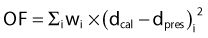
in which Σ_i represents a summation over all voxels in the PTV and w_i equals the weighting (or penalty) factor for the i^th voxel.

Usually within a PTV all voxels would have equal weighting factors, but this does not have to be true—a voxel-specific penalty scheme can, in general, significantly improve the final dose distribution because of greatly enlarged solution space.⁴²^,⁴⁷ The calculated dose equals d_cal (using the current beam parameters) for the i^th voxel. The prescribed dose equals d_pres for the i^th voxel.

The exact formulation for the objective, however, could take many other algebraic forms. For example, the absolute value of (d_cal − d_pres)_i could be used rather than its square. Or one could include (d_cal − d_pres)_i in the summation only if (d_cal − d_pres)_i is negative; that is, one must assign a penalty only if the calculated dose is less than the prescribed dose. Conversely, when calculating the contribution to the OF for normal tissue, one would usually assign a penalty only if d_cal is larger than d_pres. The total OF is then the sum of the OFs for each tissue, weighted by the w_i values, which will likely differ for each tissue. For example, one would often assign a higher penalty or weighting factor to the spinal cord than to the rectum or bladder, as the former is a more radiosensitive structure with more disastrous consequences if overdosed. Automation of the weighting factors in IP has been reported by Xing and colleagues.⁴⁸

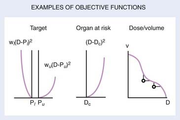
For many tissues, however, acceptable doses cannot be specified by a single dose value and dose-volume effects are often incorporated into the OF. A typical dose-volume constraint may be stated as “no more than q% of the particular organ may receive a dose greater than d.” This is equivalent to specifying a single point on a DVH with the constraint that the value of the DVH at a dose value of d must be less than q%. Most inverse treatment planning algorithms allow the planner to define multiple such points for each tissue, with different penalties assigned to each point if desired. DVH type constraints, rather than a single dose limit can also be assigned to the PTV if desired.

Several OFs are illustrated graphically in Fig. 10-7. For the PTV or target, the graph illustrates the concept of the “allowable inhomogeneity.” That is, if the dose is between a lower limit P_l and an upper limit P_u, no penalty is assessed. Also, a larger weight can be assigned to penalize underdose as opposed to overdose (or vice versa). For normal tissue, a penalty can be applied if the dose exceeds a certain critical value (D_c) or is based on dose-volume considerations, as represented schematically in the rightmost graph of Fig. 10-7.

FIGURE 10-7 • Examples of possible objective functions, illustrated graphically. For the planning target volume (leftmost graph) doses within the “allowable inhomogeneity” are permitted, with different penalties assessed for underdose as opposed to overdose. For the normal organ, a penalty can be applied if the dose exceeds a certain critical value (D_c) (middle graph), or based on dose-volume considerations (rightmost graph).

Thus dose constraints are the prescribed dose and allowable dose inhomogeneities to the PTV plus the dose limits to various sensitive structures, specified by the treatment planner to the IP computer system. The resultant inverse plan depends on the specification of these constraints. Overly relaxed or overly restrictive constraints may lead computer optimization to produce an inferior plan. In particular, if one specifies dose constraints that are physically impossible (for example, prescribing a 100% dose to a paraspinal tumor with a large penalty for underdose, plus a 5% dose to an adjacent section of spinal cord with a large penalty for overdose), the resultant inverse plan may be worse than a conventional plan. The reason for this seemingly incongruous result is that the optimization algorithm may attempt to adjust beamlet weights to extreme values in a futile attempt to meet dose constraints that are physically impossible.

To specify realistic dose constraints, users need to learn the relationship between the dose constraints and the resulting dose distributions for the specific IP system they are using, plus have some familiarity with basic radiation dosimetric concepts. This learning process is one of trial and error, and is less intuitive than the trial and error planning process involved in 3D-CRT planning. Once the treatment planner has gained this experience, it becomes possible to develop disease-specific templates that can be used as starting-point dose constraints for commonly treated tumor sites such as the prostate,⁴⁹^,⁵⁰ the nasopharynx,⁴⁵ and the oropharynx.⁵¹ Patient-to-patient anatomic variations obviously limit the use of standard dose constraints, but they can be good starting points.

Once the dose constraints are given to each type of tissue or organ, computer optimization alters the intensity of each beamlet until the OF (e.g., see equation) is minimized. The computational algorithms such as the downhill gradient method or the simulated annealing method are often used to expedite the search of the minimum.

Generation of Leaf Motion Files

The “leaf sequencer” is an algorithm within the IMRT planning system that translates the beam intensity pattern produced by the IP system into an instruction set describing how to move the MLC leaves during beam delivery. Depending on the specific IP system being used, the result of optimization may be either continuous 2-D intensity profiles, or discrete 2-D intensity matrices with discrete resolution, such as 10 mm × 1 mm spatially, with 5% intensity steps. The term DMLC delivery (often referred to as a sliding window) delivers a continuous 2-D intensity profile, whereas static delivery (often referred to as step and shoot) results in “discretized” intensity patterns.

There are many possible sequences of dynamic leaf motions (or equivalently, combinations of multiple static field segments) capable of producing a desired intensity pattern because the problem of leaf sequencing is underdetermined mathematically.¹⁵ Depending on the delivery method, algorithms have been developed to minimize the number of segments, the number of total MUs, the leaf travel distance, and the total delivery time.⁵²^–⁵⁷ Here, we describe one basic leaf sequencing method using DMLC (sliding window).

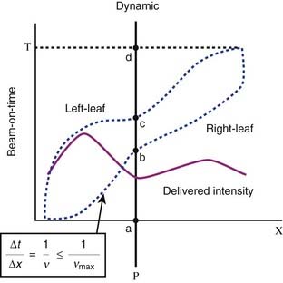
This leaf sequencing method ⁵⁴ divides the 2-D intensity distributions into a number of one-dimensional intensity profiles, with each profile delivered by one pair of leaves. The leaf paths are illustrated in Fig. 10-8, which shows a schematic representation of radiation delivery using the sliding window method. The dotted lines represent the positions of a leaf pair (x-axis) as a function of beam-on time (y-axis). Both leaves start at the extreme left edge of the intended treatment field. As the beam is turned on (a), both leaves move at different speeds from left to right (initially the right leaf moves more rapidly than does the left leaf). The point P begins to receive radiation when the right leaf edge moves past it (b), and continues to receive radiation until the left leaf blocks the beam (c). By controlling the movement of the leaves and therefore the “beam-on-time” duration between b and c, one can deliver any desired intensity to point P, or any other point under this leaf pair. The solid line depicts the total integrated beam intensity to all points underneath the strip of tissue being treated by this leaf pair.

FIGURE 10-8 • Schematic representation of radiation delivery using the sliding window method. The dotted lines represent the positions of a leaf pair (x-axis) as a function of beam-on time (y-axis), and the solid line depicts the total integrated beam intensity to all points underneath the strip of tissue being treated by this leaf pair. See text for details.

By extending this concept to multiple pairs of leaves, any desired intensity-modulation pattern can be produced with designed sequences of leaf positions. Because each leaf pair must deliver a different intensity profile, the speed of each leaf and its position as a function of MUs delivered must be individually controlled. For maximum efficiency in beam delivery (i.e., shortest possible treatment times), it is necessary to be able to move all leaves simultaneously. This requires both leaf speed modulation and dose-rate modulation. Ideally, one would always treat at the maximum dose rate of the linear accelerator, but when a leaf is required to move a large distance, requiring a speed exceeding the maximum mechanical leaf speed, the dose rate must be reduced. In practice, not all desired intensity profiles are exactly achievable because of the constraints on leaf motion imposed by the design of the MLC and the clinical dose rate of the machine. The details of MLC design limitations on IMRT delivery are discussed more fully in “Delivery of Intensity-Modulated Treatment,” in this chapter.

Direct Aperture–Based Optimization

The typical pixel-based or fluence-based (described previously) IP optimization often results in complex IMRT plans, which prolongs the treatment time and dramatically increases the number of MUs by two to five times.⁵⁸ The latter could lead to increased leakage and scatter radiation through the MLC, and this indirect radiation contribution has been shown to adversely affect the accuracy of treatment delivery.⁵⁹ More importantly, the increased exposure from complex IMRT plans may also increase the frequency of radiation-induced secondary malignancies. It has been recently reported that the transition from 3D-CRT to IMRT resulted in a larger volume of normal tissue exposed to a low dose of radiation, which was estimated to increase the incidence of secondary cancers at 10 years from 1% to 1.75%.⁶⁰

The complexity of IMRT plans originates not only from the use of pixel-based or fluence-based optimization, but also from the separation of leaf sequencing from the optimization, referred to as a two-step process. During leaf sequencing, the computer program may generate many small area segments (or subfields) to avoid significant deviation from the initially optimized plan. The use of these small area segments in IMRT plans significantly reduces overall efficiency of radiation and may introduce additional dosimetric errors. Based on our local institutional plan acceptance criteria, this type of optimization typically results in a total number of segments ranging from 100 to 180 for head and neck IMRT plans, and a total number of segments ranging from 60 to 100 for prostate-only IMRT plans.

To simplify IMRT plans (or avoid overly complex IMRT plans) while improving delivery and radiation efficiency, many researchers have been working on increasing the efficiency of leaf sequencers.^55,^57,⁶⁰^–⁶³ Some leaf sequencers minimize the total number of segments, whereas others minimize the total required MUs. Other researchers have proposed the use of smoothing filters to eliminate unnecessary noise inside the intensity profiles, either during optimization or prior to leaf sequencing.⁶⁴^,⁶⁵ With most commercial planning systems, options for controlling the complexity of an IMRT plan are often limited to choosing coarse intensity levels during conversion, selecting a leaf sequencer that can provide an optimal delivery efficiency for the specific delivery method (e.g., sliding window or step-and-shoot methods, discussed further in “Static Versus Dynamic Multileaf Collimator Delivery,” later in this chapter), or using smoothing filters.⁶⁶^–⁶⁸ However, the effectiveness of these methods in controlling the complexity of an IMRT plan is limited, often resulting in significant deteriorations in plan quality.