Three-Dimensional Conformal Radiation Therapy
Karl L. Prado
George Starkschall
Radhe Mohan
Introduction
The goal of radiation therapy is to irradiate tumor-bearing tissues while sparing normal structures. Specifically, we would like to deliver a dose of radiation to tumor cells that is large enough to produce cell kill at a sufficiently high probability level to control malignant disease, while at the same time limiting the dose to uninvolved surrounding tissues so that the probability of inducing damage to these tissues is kept to a minimum. In external-beam radiation therapy, in which beams of radiation necessarily traverse normal tissues in order to treat tumor-bearing anatomic sites, this goal is often difficult. At dose levels at which tumor control becomes reasonably probable, normal tissue damage becomes a serious consideration.
The primary obstacles to achieving the maximum possible therapeutic advantage in favor of the patient being treated with conventional radiotherapy are the following:
The uncertainties in the true spatial extent of the disease
Inadequate knowledge of the exact shapes and locations of normal structures
The lack of optimal tools for efficient planning and delivery of conformal radiation therapy (CRT)
limitations of existing methods of producing desirable radiation dose distributions
These limitations result in the incorporation of large safety margins to reduce the risk of local relapse. However, to ensure that unacceptable normal tissue complications are prevented, the tumor dose often has to be maintained at suboptimal levels, leading to a higher probability of local failures. Therefore, better localization of the extent of the tumor and of normal critical structures and the ability to shape the dose distributions accordingly are essential to reduce the margins, allowing increases in tumor doses and minimizing dose to normal tissues.
Consider a common treatment-planning scenario, in which a tumor lies within a region of uninvolved tissue, and a uniform dose of radiation is delivered to the site. As the dose delivered to this site increases, the probability of tumor control increases, as does the probability of inducing normal tissue damage (Figure 12.1). Depending upon the dose–response characteristics of the tumor and of the surrounding normal tissues, it may not be possible to control the disease at a high enough probability level, without also producing normal tissue damage. Therefore, it very often becomes necessary to deliver higher doses to the tumor than to the surrounding uninvolved tissue. This is accomplished by selectively targeting tumor volumes with multiple radiation beams.
Despite considerable progress in improving the accuracy and precision of radiation therapy, many sources of uncertainty remain. These include the limitations of imaging devices to reveal the true extent of the disease, displacement of the internal anatomy at the time of treatment relative to its position at the time of imaging, motion of patient and internal organs during treatment, variation of response to dose from one patient to the next, intratumor variation in response, dosimetric inaccuracies, and so on. These are complex problems, but a reduction in uncertainties is essential for the accumulation of more accurate data and for an improvement of the state of the art of radiotherapy. A considerable amount of effort is being devoted to reducing uncertainties.
Targeting for Three-Dimensional Conformal Radiation Therapy
The process by which external beams of radiation are designed and used to selectively and exclusively irradiate only tumor-bearing sites is called three-dimensional conformal radiation therapy (3-DCRT). In 3-DCRT, tumor sites are meticulously identified, as are normal structures considered at risk of damage. A treatment plan is created in which radiation beams are carefully designed to include only tumor sites while excluding, as best possible, normal structures considered at risk. The resulting dose distribution is calculated and evaluated in light of dose–response criteria established for the disease and for normal structures at risk. Once approved, the plan can be delivered.
In this chapter, the process of 3-DCRT is reviewed. Initially, necessary terminology is defined. Methods for defining and recognizing tumor-bearing volumes are then described. The rationale for designing radiation-beam portals is explained, emphasizing the concept of margins. The process by which dose distributions are produced and analyzed is then described. Finally, delivery and verification of 3-DCRT are discussed.
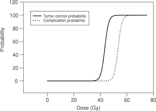 Figure 12.1. Schematic representation of the dependence of tumor control probability (TCP) and normal-tissue complication probability on dose. The shape of the curve and its position on the dose axis vary. In the scenario shown here, a relatively high TCP can be achieved at dose levels where the probability of normal tissue complications is low. This is very often not the case. In fact, in many instances, normal tissue complications occur at dose levels below those at which tumor control is probable. |
International Commission on Radiation Units and Measurements Definitions
3-DCRT has been demonstrated to be a viable method for achieving high precision in radiation therapy. In addition to the geometric precision achievable by 3-DCRT and the dosimetric precision achieved by standardized dosimetry protocols, such as the TG-51 protocol (1), modern radiation oncology needs correspondingly high precision in specifying the radiation dose prescription and the resulting dose distributions. Moreover, when communicating radiation treatment information, for example, in interinstitutional treatment protocols, unambiguous definitions of dose and dose delivery are needed.
The International Commission on Radiation Units and Measurements (ICRU), in a series of reports (2,3), has defined various volumes to support this need for precision and absence of ambiguity in the definition of dose delivery. Two reports have already been written, and it is likely that more may be forthcoming.
The ICRU has defined several regions related to the tumor. The gross tumor volume (GTV) is defined to be the “gross demonstrable extent and location of the malignant growth” (2). The GTV may include primary tumor, involved lymph nodes, and metastatic disease, and is demonstrated using whatever imaging modalities are appropriate, whether it be by visual observation, computed tomography (CT), magnetic resonance imaging (MRI), positron emission tomography (PET), single photon emission computed tomography (SPECT), or by any other method of visualization. Some ambiguity exists in the delineation of the GTV, as different imaging modalities may display different extents of disease. Moreover, differences in image quality such as spatial resolution, temporal resolution, and contrast-noise ratio may result in differences in the way in which a tumor appears, resulting in differences in the delineation of the GTV. The patient may have several GTVs, depending on the extent of disease, and the treatment goals for each GTV may be different. Furthermore, following surgical intervention, it is possible that the GTV may not necessarily be present.
In addition to the demonstrable disease, the patient is likely to have subclinical disease that is known to be present. The demonstrable tumor plus the microscopic disease constitute the clinical target volume (CTV). The margin surrounding the GTV that defines the CTV is delineated based on clinical experience, or in some cases, pathology studies. In the case where surgical intervention has taken place before radiation treatment and the GTV has been removed, a CTV may exist in the absence of a GTV. The goal of the radiation therapy is to irradiate the CTV to a dose appropriate to control the disease. The GTV and CTV are based on oncologic principles and are not restricted to radiation therapy. For example, the CTV can be the volume defined for surgical resection. Both the GTV and the CTV are defined before any planning for radiation treatment.
In conventional 3-DCRT, the GTV and CTV are based on imaging information acquired several days before treatment. This information is assumed to be an accurate representation of the patient for the entire course of radiation therapy. Patients, however, may change during treatment as a result of factors including gain or loss of weight, bladder, or rectal filling, or changes in the size of the tumor. Intrafractional changes may also occur during an individual radiation treatment due to various physiologic motions such as respiratory motion, cardiac motion, peristalsis, and swallowing. Margins are needed to surround the CTV to ensure that the CTV lies within the treatment field during the entire course of radiation therapy. These internal margins (IMs), in addition to the CTV, constitute the internal target volume (ITV). ITVs can be delineated as a result of IMs implicitly determined based on population studies, or can be explicitly determined by the use of various types of motion studies, often based on acquisition of multiple CT images.
Finally, in order to account for setup uncertainties, one adds a setup margin (SM) to the ITV to generate a planning target volume (PTV). The SM for a specific treatment is generally based on population studies and methods of immobilization. Invasive immobilization techniques such as a stereotactic head frame may result in submillimeter SMs, although other immobilization methods may yield SMs of several millimeters. The PTV is the final volume that must be irradiated to the tumoricidal dose to ensure that the CTV is actually irradiated to the desired dose. If not all the PTV has been irradiated, then the possibility exists that the CTV might not receive the appropriate dose. In the planning of 3-DCRT, beam apertures are designed to ensure complete irradiation of the PTV, whenever
possible. Figure 12.2 illustrates an axial CT image with GTV, CTV, and PTV identified and delineated.
possible. Figure 12.2 illustrates an axial CT image with GTV, CTV, and PTV identified and delineated.
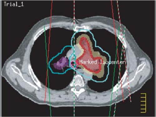 Figure 12.2. The gross tumor volume (GTV), clinical target volume (CTV), and planning target volume (PTV) of patient with lung cancer. The hilar GTV is shown in red color wash surrounded by a thick-line red contour. The CTV extends 8 mm beyond the GTV and is shown in brown color wash. The PTV extends 7 mm beyond the CTV and is represented by the light blue contour. On the patient’s right, second CTV and PTV are similarly shown. |
In addition to ensuring adequate dose delivery to the PTV, the treatment plan must also account for the presence of uninvolved tissue, which, if given excess radiation, might be damaged, compromising the success of the radiation treatment. The ICRU defines an organ at risk (OAR) to be an organ that, if given an excess radiation dose, would compromise the success of the course of radiation therapy. The identification of the OAR is based on the site to be treated. For example, for thoracic treatments, OARs include each lung, the heart, esophagus, and spinal cord. Organs not likely to be irradiated in the course of radiation treatment are not considered to be an OAR for that treatment.
Just as the CTV must be expanded to account for setup uncertainty and organ motion to generate a PTV, so must the OAR volume be expanded to account for setup uncertainty and organ motion to generate the planning at risk volume (PRV). In some cases, the PTV and PRV might overlap, but often treatment planning is a set of compromises between full irradiation of the PTV and overirradiation of the PRV. Radiation oncologists and treatment planners need to be fully aware when such compromises are being made. It is not correct to make changes in any of the target volumes or the PRVs to make the treatment plan appear better; these volumes must be determined before the plan is developed. If a PTV is to be reduced, some justification needs to be given, such as more precise imaging to reduce the GTV or more precise immobilization to reduce the PTV. Sometimes nonstandard margins may be specified around a PTV or a PRV for the purposes of optimization, but these margins should only be used for the optimization and not be reported in the final assessment of the radiation treatment plan.
Imaging in Three-Dimensional Conformal Radiation Therapy
Accurate methods of imaging play an essential role in the successful implementation of 3-DCRT. Patient images of various types are used in every step of the 3-DCRT procedure. These images may be cross-sectional or projections, and they may come from one or more of various modalities. Before the 3-DCRT era, imaging patients for treatment planning consisted of acquiring one or more cross-sectional images on a CT scanner as well as planar images on a conventional simulator. The conventional simulator was a radiographic/fluoroscopic unit with gantry and collimator motions that simulated those of the radiation treatment machine. Gantry angles were either determined from a plan generated from the CT image or based on class solutions, and then simulated on the conventional simulator. Treatment portals were determined primarily based on two-dimensional (2D) internal anatomy, where known and suspected disease was targeted and critical structures were avoided.
The present state of 3-DCRT practice involves CT-based simulation. Because of the availability of CT scanners capable of high-speed image acquisition and reconstruction, and possessing abundant and inexpensive memory, patient images are now acquired on axial planes with resolutions of 3 mm or less, allowing for accurate volumetric determination of targets and normal anatomy. Treatment planning is then based on 3D anatomy, with design of beam geometries and treatment portals based on the 3D extent of defined targets and normal anatomy. In CT simulation, a 3D CT image set of the patient is obtained in the treatment position. Patients are placed in some form of immobilization device and are appropriately marked to ensure setup reproducibility. Setup reproducibility may vary from submillimeter accuracy in the case of stereotactic and hypofractionated treatments in the head or central nervous system, where critical structures may lie in close proximity to the target volume, to accuracies of 0.5 to 1 cm for some regions of the thorax, abdomen, or extremities.
Various generations of CT scanners have been used to acquire patient information for 3-DCRT. The advent of the third-generation CT scanner, which consists of a single radiation source detected by a single fan-shaped array of radiation detectors, has made image acquisition time sufficiently rapid to make 3-DCRT image acquisition practical. In a third-generation CT scanner, the gantry makes a single (whole or partial) rotation around the patient. The transmission pattern of a single slice is acquired by the array of detectors and is reconstructed. After acquisition of a single slice, the patient table is indexed and another slice is acquired. This procedure continues until the entire 3D CT image has been obtained. The newer technology of helical, or spiral, CT combines gantry rotation with table translation, so that the path of the radiation source makes a spiral trajectory. Coalescing table translation with
gantry rotation in this manner significantly speeds up the acquisition of the CT image information. To speed up image acquisition even further, detectors and reconstruction algorithms have been developed that allow acquisition and reconstruction of multiple axial CT slices at one time. This technique of multislice helical CT image acquisition has the potential for scan times as short as 3 to 5 seconds (4). Multislice helical CT scanners used in combination with respiratory monitoring and triggering methods also allow capture of respiratory-induced motion in what is now referred to as “four-dimensional” CT scanning (5,6).
gantry rotation in this manner significantly speeds up the acquisition of the CT image information. To speed up image acquisition even further, detectors and reconstruction algorithms have been developed that allow acquisition and reconstruction of multiple axial CT slices at one time. This technique of multislice helical CT image acquisition has the potential for scan times as short as 3 to 5 seconds (4). Multislice helical CT scanners used in combination with respiratory monitoring and triggering methods also allow capture of respiratory-induced motion in what is now referred to as “four-dimensional” CT scanning (5,6).
The ability to acquire CT scans with high axial resolution accentuates the question of optimal axial resolution for 3-DCRT planning. Before 3-DCRT, CT image data sets were acquired at axial separations of 10 mm or more. In principle, the axial resolution should be similar to the resolution of a picture element (pixel) in a transverse plane of a CT image, which is somewhat <1 mm. However, such fine axial resolution would result in the production of a very large number of CT images in a data set. Delineating target volumes and normal anatomic structures on such large number of images would significantly increase the time required to develop patient treatment plans, as the contouring process is presently very labor intensive. Effective and efficient contouring tools, as discussed later in this chapter, may be of significant assistance in this process, allowing higher axial resolution image data sets to be incorporated into 3-DCRT planning, but at present, axial resolutions of 2 to 3 mm appear to be the acceptable standard.
Images used in 3-DCRT consist of pixels with a large range of CT-number values. Pixel values in CT images, for example, are normally stored as 12-bit unsigned integers, allowing values from 0 to 4,095. Typically, pixel values are binned into a significantly smaller range of gray-scale values for display. Through appropriate selection of binning methods, one may be able to enhance features of images, possibly enabling better recognition of tumors and anatomic structures. The simplest and most frequently used image enhancement method is that of windowing and leveling. Instead of distributing the entire range of pixel values evenly across the gray-scale spectrum, one selects a window, that is, a limited range of pixel values for display, and a level, which is the location of the window. For example, one could select a range of pixel values between 900 and 1,100 for display. This would be a window of 200 at a level of 1,000. All pixels with values lower than 900 would be displayed as black, and pixels with values greater than 1,100 would be displayed as white. Pixels with intermediate values would then be displayed as shades of gray. Increasing the window width would decrease the contrast of the image; decreasing the window width would increase the contrast of the image. Figure 12.3 illustrates two CT images of an axial slice of a patient’s thorax. The figure on the left displays the image using a window typically used to display mediastinal structures, with a window level of 1,060 and a width of 400 (i.e., a range of pixel values from 800 to 1,200), whereas the figure on the right displays the same image using a window typically used to display lungs, with a window level of 500 and a width of 1,600. Note the significantly different contrast in the two images. This may lead to differences in the way tumors are delineated, so it is important that a consistent set of windows and levels be used for tumor delineation in any one site.
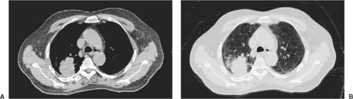 Figure 12.3. An axial computed tomography (CT) image of the thorax, shown in “mediastinal” (A) and “lung” (B) windows. The pixel values included in the mediastinal window range from 800 to 1,200; those of the lung window range from 300 to 1,300. |
In windowing and leveling, the interval of pixel values is divided into equally spaced subintervals, each subinterval being assigned a specific gray-scale value. It is possible, however, that the pixel values in an image may cover a wide range, but the vast majority of pixels may be concentrated in a narrow range and have values less than the average. The details in the darker regions of such images may be difficult to perceive. If the pixel values are divided into bins of equal width and a histogram of the number of pixels in the bins against the pixel value is drawn, it will be sharply peaked, with the peak near the lower end of the intensity range. An alternative method of binning pixel values known as histogram equalization allows pixel subintervals of variable width with the requirement that an equal number of pixels are binned into each subinterval. This technique can be of significant utility for images for which there might be a bimodal distribution of pixel
values. It is more commonly used to enhance portal images rather than CT images.
values. It is more commonly used to enhance portal images rather than CT images.
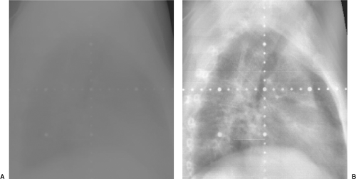 Figure 12.4. Portal image of a lateral chest without image enhancement (A) and with histogram equalization (B). |
An extension of the histogram equalization technique is adaptive histogram equalization (AHE). In AHE, the contrast of each pixel is adjusted according to histograms of pixels in the immediate vicinity of the pixel rather than the histogram of pixels in the entire image. This scheme optimizes the contrast by assigning brightness in the local context. Typically, a 64 × 64 subimage histogram is selected. Variations of AHE, for example, clipped, or contrast-limited AHE (CLAHE), have also been proposed to enhance the images further (7,8). Although AHE and its variants are not yet used extensively in radiation oncology, they have the potential to reveal a great amount of anatomic detail and to aid in the laborious task of manual segmentation as well as in the automatic extraction of anatomy. Histogram equalization techniques are frequently used to evaluate portal images, which tend to be severely lacking in contrast. Figure 12.4 illustrates two portal images of a lateral thoracic field. In the image on the left, only the window and level have been adjusted for clarity, but no other modifications have occurred, whereas in the image on the right, AHE has been applied to improve the clarity of the image. Features that are barely visible on the conventional portal image are quite readily displayed on the histogram-equalized image.
In another form of contrast enhancement, images may be filtered to sharpen their edges. A variety of filters are available. Some filtration techniques use Fourier transforms to convert the image into the frequency domain. In the frequency domain, the rapidly changing features (e.g., the edges) are transformed into higher-frequency components. Reducing the amplitude of lower-frequency components and converting the image back into the spatial domain would enhance the edges of the image. This is called high-pass filtration. Other edge enhancement filters, for example, Sobel (9) and Canny (10) filters, use gradient techniques. In some instances, the gradient image showing only the edge information can be obtained.
Gross Tumor Volume Determination
Imaging is used extensively in the definition of 3-DCRT target volumes. Identification of exactly what is to be treated is perhaps the most important component of the 3-DCRT process. To assist in this determination, target and treatment volumes have been clearly defined by the ICRU and have been amply described previously in this chapter. The ICRU definition of the GTV, the “… gross demonstrable extent and location of malignant growth …,” (2) highlights an important characteristic of this volume, namely that it is “demonstrable,” or readily shown or proved. Evidence that a tissue volume contains tumor can be obtained from multiple sources. Among these sources of information are clinical examination, such as palpation, and the use of imaging techniques. Except in circumstances where tissues can be readily observed with the naked eye or palpated directly, imaging is used to define the GTV.
Given the recent advances in imaging technology wherein functional imaging is finding an increasingly significant role in tumor volume definition, the traditional definition of the GTV is undergoing a change (11). The explicit use of 18F fluorodeoxyglucose (18FDG) PET imaging, for example, as
an aid in defining the GTV, now reveals tumor-bearing tissues that may have been previously occult, excluded from the GTV, and therefore are considered part of the CTV. This issue is discussed in more detail in a later section of this chapter. In this next section, the use of images to define the GTV is explored.
an aid in defining the GTV, now reveals tumor-bearing tissues that may have been previously occult, excluded from the GTV, and therefore are considered part of the CTV. This issue is discussed in more detail in a later section of this chapter. In this next section, the use of images to define the GTV is explored.
Image Segmentation
Image segmentation is the process by which pixels within an image are identified and classified based on specific properties. Pixels are identified on the basis of their appearance (e.g., density, texture, or pixels bounded by an edge). They can be classified as belonging to a group or class defined as a particular organ system, such as lung, or they can be defined as belonging to a group identified as GTV, or both. For specific applications in radiation treatment planning, the term image segmentation is used to describe the task of manually or automatically delineating anatomic regions of interest, including critical normal organs and the target volume, on the 3D patient image. Accurate information about the shapes and locations of anatomic structures is essential for aiming beams at the target volume while minimizing the exposure of normal tissues. Segmented structures are also necessary for the qualitative and quantitative evaluation of treatment plans using dose distribution displays, dose–volume histograms (DVHs), and predicted values of biologic indices. In addition, anatomic structures overlaid on digitally reconstructed radiographs (DRRs) are important for correlating the planning geometry with the treatment geometry using DRRs and portal images.
The process of image segmentation is perhaps the most labor-intensive component of 3-DCRT, as pixels must be individually identified as belonging to one or more groups or classes. The identification process can be either automatic or manual. For many anatomic structures of interest, the contrast near the boundary of the structures is sufficient for automatic edge-detection schemes—often times, it may not be. When automatic edge-detection routines fail to properly identify differences in tissue classification, manual means must be employed. In these instances, outlines must be drawn by guiding the cursor on the image with a mouse, trackball, or light pen. For target volumes, one must delineate a region that includes the gross disease, regions of known extensions, and regions of suspected disease. The latter two are not likely to be discernible on images, and the boundary has to be drawn according to prior knowledge and experience. Considering the arduousness of the task, efficient manual drawing tools are crucial to the success of 3-DCRT.
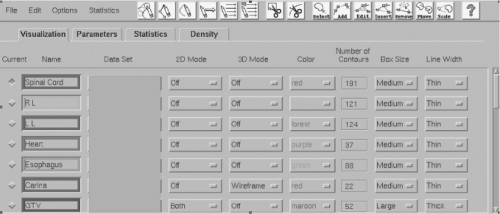 Figure 12.5. Contouring tools that are routinely available in modern treatment-planning and virtual-simulation software are shown in the top toolbar of this contouring panel. Contours can be drawn in a point-by-point or continuous fashion, using “pencils” or “brushes.” Contours can be cut, copied, and pasted, as well as edited, moved, and scaled. The resultant regions can then be visualized in multiple colors using various rendering techniques (see text). |
Many different software tools have become available for accelerating and simplifying the task of manually drawing contours. The choice of the pointing device (e.g., mouse, trackball, light pen) may affect productivity. Tools such as “pencils” and “brushes” of various sizes can also be used to identify individual pixels or groups of pixels and to conform contours to structures (Figure 12.5).
The various image enhancement techniques discussed earlier can be used to maximize the visibility of anatomic detail for manual contouring. The automated selection of the most appropriate enhancement techniques and their parameters for each class of anatomic structure and treatment site can save a significant amount of time and effort. Often anatomic structures, including target volumes, do not vary significantly from one image section to the next. Therefore, a tool to copy contours drawn on the adjacent section and to reshape them can be effective. Another useful capability is the interpolation of contours. Contours drawn on a limited number of widely separated image sections can be interpolated to generate contours on intervening image sections and edited if necessary. The
efficiency of manual drawing and editing also depends greatly on the user interface and its adaptability to individual user preferences and to individual classes of problems. In general, the best interfaces are those that allow the user to enter and edit the information with a minimum of cursor motion, mouse clicks, and keystrokes.
efficiency of manual drawing and editing also depends greatly on the user interface and its adaptability to individual user preferences and to individual classes of problems. In general, the best interfaces are those that allow the user to enter and edit the information with a minimum of cursor motion, mouse clicks, and keystrokes.
Although improvements in the manual drawing of contours continue, there is also a need to develop robust techniques to segment anatomic structures automatically. For anatomic structures that appear as high-contrast objects on images, the problem has mostly been solved with the aid of edge detection and edge tracking techniques. Examples of structures that may yield to edge tracking techniques include the boundary of the skin, lungs, bony structures, and cavities in the head and neck. In techniques of this type, the computer automatically tracks the path of a specified pixel value and connects the pixels into a contour outline. To minimize the effect of noise in the image data to obtain a smooth curve, pixel values are averaged over a neighborhood of specified dimensions. In some instances (e.g., for skin and lungs), the computer can be programmed to use some easily definable logic to detect the starting position automatically; in other instances, the starting position may have to be set by the user. Edge tracking may be extended to three dimensions, in which outlines of the specified anatomic structure on all image sections are automatically detected. In one such extension for lung, the position of the centroid of the contour on one image section is used to seek the lung interface on the next image section. Unfortunately, 2D or 3D edge-detection techniques do not always succeed even for such seemingly simple cases as skin and lung, so manual intervention is required. In particular, if the anatomic structure being segmented is not completely surrounded by voxels with a significantly different CT number, edge-detection techniques will fail to generate a reliable contour. Figure 12.6 illustrates this problem. In Figure 12.6, a right lung is auto segmented using an edge-detection algorithm that detects edges with a CT number of 800. In Figure 12.6A, the right lung is correctly segmented, but in Figure 12.6B, the segmentation also included the left lung. The left lung was included because the tissue separating the right and left lungs was not of sufficiently high density. The failure rate of edge-detection techniques is of the order of a few percent for high-contrast objects but is enough to require review of all automatically drawn contours. Edge detection may be supplemented with edge enhancement and thresholding. Thresholding may be used to highlight pixels in a given range of values. The range is adjusted during visual inspection of all image sections of interest. Any stray pixels and areas of potential problems may be edited away before automatic edge detection is attempted. Even though a modest amount of manual intervention is needed, the process is quite accurate and reliable.
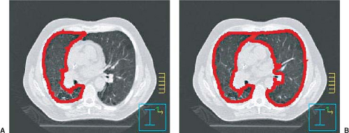 Figure 12.6. Results of autosegmentation of a patient’s right lung. A: A successful autosegmentation search using edge detection with a threshold computed tomography (CT) value of 800. B: An unsuccessful autosegmentation in which the edge detection failed as a result of inadequate separation between the right and left lungs. |
The standard edge-detection techniques may work reasonably well for high-contrast objects; however, they perform poorly for objects with medium contrast and with edges that are diffuse and which are only partially visible. For delineating these objects, considerable attention is being focused on more sophisticated automated and semiautomated methods to fill the gaps in the edge information. It is unlikely that any general solution will be found, and a custom solution for each anatomic structure may have to be developed. A promising approach is the so-called deformable model technique (12,13). In this technique, the image is preprocessed with pixel and texture classification and edge enhancement to identify any edges and clusters of pixels belonging to the object. The edges, pixels, and pixel clusters are used to deform the surface of a model of the anatomic object. The model surface is represented by a series of connected polygons obtained by averaging the manually drawn shape of the organ over a group of patients. Deformation is carried out by forces
applied to each polygon in an attempt to minimize an energy functional. The energy functional consists of two terms, an “internal” term that tends to smooth the surface of the anatomic structure, and an “external” term that tends to fit the surface of the anatomic structure to the intensity edges in the image. Application of the deformable model technique to CT image segmentation in the pelvis has been described by Pekar et al. (14) and that in the thorax by Ragan et al. (15).
applied to each polygon in an attempt to minimize an energy functional. The energy functional consists of two terms, an “internal” term that tends to smooth the surface of the anatomic structure, and an “external” term that tends to fit the surface of the anatomic structure to the intensity edges in the image. Application of the deformable model technique to CT image segmentation in the pelvis has been described by Pekar et al. (14) and that in the thorax by Ragan et al. (15).
The ability to segment an anatomic structure automatically may also depend on the imaging modality. MRI, for instance, provides a much greater contrast in the brain and central nervous system; CT is more appropriate for outlining bony anatomy. Therefore, there is often a need to merge information derived from one imaging modality with that from another. This topic is discussed in detail in the next section.
Image Registration and Correlation
The CT image set comprises the fundamental dataset within which anatomy and targets are defined, dose is computed, and treatment plans are evaluated. This is due to its prevalence as an imaging modality, its high spatial resolution and accuracy, and its necessity for dose computation, as the pixel values can be directly correlated to the interactions of the radiation with tissue. In modern computer systems used for treatment planning, the CT dataset of the patient serves as the basis for the establishment of the spatial coordinate system that will be subsequently used for registration of anatomy and radiation-beam targeting. The CT dataset, therefore, can be thought of as a 3D matrix representing the patient’s anatomy. Within this image matrix, volume elements, or voxels, indicate the coordinates of the element, and contain the elements’ CT numbers. Additional characteristics can be assigned to these matrix elements as the treatment-planning process progresses. Such characteristics include identification of the element as belonging to a tissue class (such as lung or spinal cord), target group (such as GTV), and dose value (once beams are placed and dose is computed).
As mentioned previously, during the initial phases of the planning process, images are segmented to identify targets and normal tissues. All possible sources of information are used to more accurately define these structures. No single imaging modality may produce all the information needed for the accurate identification and delineation of the target volume and critical organs. Different imaging modalities produce visual renditions of different processes. MRI, for instance, produces images in which the gray scale represents either proton density or proton relaxation times, a characteristic of the chemical environment of the voxel. MRI is well suited for imaging the central nervous system, sarcomas, head and neck cancer, and prostate cancer, as well as for the visualization of lymph nodes. PET with 18 fluarodeoxyglucose (18FDG) produces images in which gray scale is assigned values proportional to the degree of uptake of FDG by the tissue. The uptake is in turn a function of metabolic activity. Therefore, PET provides metabolic and functional information that may be useful in determining the extent of the tumor, in particular, its microscopic spread. Each unique piece of information needed for the planning and delivery of radiotherapy should ideally be derived from the most suitable source, and then integrated into the CT image set.
Often, the transfer of anatomic and physiologic information is accomplished by manual drawing during visualizations of both sets of images side by side. This process is laborious, approximate, and not particularly well suited for 3-DCRT. Necessary automated methods to assist in image registration are evolving rapidly. Registration of 3D images entails the computation of a transformation function that accurately registers information derived from one 3D image data set to another. The transformation function depends on whether the two sets of images are related through only rigid body transformations, namely, rotations and translations, or whether individual anatomic structures have been deformed or displaced relative to each other. The case of rigid body transformation is much simpler but is accurate in only select circumstances. In essence, a combination of clearly identifiable points, lines, surfaces, and images of anatomic landmarks and external fiducial markers on two data sets are identified and used to match and correlate them. Various techniques, such as cross-correlation (16) or mutual information (17) may be used to obtain the transformation function between the coordinate systems of the two sets. The transformation function is typically a 4 × 4 matrix describing three rotations, three translations, and perhaps simple scaling. This matrix may be used to transform any point or a collection of points (e.g., pixels and contours) on the image correlated to the reference image. Once transformed, the correlated image may be “resliced” to produce image sections in the same coordinate system as the reference image for the side-by-side display and comparison. The outlines and surfaces of anatomic structures abstracted from the correlated image may be transformed to the reference image using the transformation matrix.
For a number of situations, the automatic matching of image data sets may be inadequate or may not be feasible. This may happen, for example, when external fiducial markers are not available, internal landmarks are not easily and accurately identifiable, or when small deformations and relative displacements of anatomic structures are present. In such situations, human judgment may be needed to match two image data sets by interactively manipulating data from both sets of images. Once a satisfactory match has been accomplished, assuming that the rigid body transformation is applicable, the transformation matrix may be computed and used.
If, however, significant deformations and relative organ displacements are present, the problem is considerably more complex. Such distortions are sometimes inherent in
the imaging devices, for example, because of inhomogeneities of the magnetic fields in the MRI. Distortions may also be caused by internal organ displacement that occurs naturally, by somewhat different positioning of the patient on different imaging and treatment devices, and by weight loss over the course of treatment. The incorporation of such distortions is a difficult task and a topic of continuing investigations.
the imaging devices, for example, because of inhomogeneities of the magnetic fields in the MRI. Distortions may also be caused by internal organ displacement that occurs naturally, by somewhat different positioning of the patient on different imaging and treatment devices, and by weight loss over the course of treatment. The incorporation of such distortions is a difficult task and a topic of continuing investigations.
A possible limited solution would be to unwarp the distorted image with image metamorphosis techniques. In techniques of this type, also known as morphing, surfaces of as many easily identifiable anatomic objects as possible are delineated on both images. A function of the distances of a pixel from various points in the identified objects is used to identify a corresponding pixel on the distorted image bearing the same relationship to the distorted objects. The pixel value at this point in the distorted image becomes the pixel value on the transformed unwarped image (18).
Clinical Target Volume Expansion
Once the GTV has been defined, it then becomes necessary to identify those areas that are suspect of containing disease. It is an accepted fact that a cancer cell population extends beyond those areas that can readily be seen or palpated. In the terminology of the ICRU (2), “… in some anatomically definable tissues/organs, there may be cancer cells at some probability level, even though they cannot be detected with present day techniques.” The subclinical disease in this extended area is commonly referred to as “microscopic disease” or “microextensions” of the disease, since confirmation of the existence of the disease in this area often requires pathologic validation with a microscope. As defined previously, the anatomic volume that contains both the demonstrable tumor (the GTV) and its associated microscopic extension is called the CTV. In the process of defining 3-DCRT target volumes, after the GTV has been identified, a margin is added around the GTV to account for the possible presence of microscopic disease. The volume produced by this extended margin in three dimensions constitutes the CTV. For other anatomic sites, for example, lymph nodes, only the presumed clinical spread of disease is used to define the CTV. These volumes may be also defined as CTVs, even though gross tumor may not be evident in the volume.
The topic of CTV definition is of considerable interest at present. In a recent and relatively comprehensive report that addresses target localization uncertainties, techniques that can be used to quantify GTV-to-CTV expansions are discussed (19,20). The nature and extent of the GTV-to-CTV expansion is based on the particular disease’s pathology. It is an area of much needed research, as available data are sparse. Given the definitions of the terms GTV and CTV, the exact extent of malignancy beyond what can be seen or demonstrated has to be determined. This validation can only be accomplished through pathologic examination of tissue specimens after they have been imaged in vivo. For example, Giraud et al. report the results of the measurements made of the extent of micro-invasion of non-small-cell adenocarcinoma and squamous cell carcinoma of the lung (21). In their study, the investigators contoured on CT, the lung tumors of patients that subsequently underwent surgical resection. The microscopic extent of the disease was determined by pathologic evaluation, and this extent was then spatially related to the contours previously drawn. They concluded that in 95% of the patients studied, adenocarcinomas extended 6 mm and squamous cell carcinomas extended 8 mm beyond the CT-based contour. In a similar study, Apisarnthanarax et al. (22) measured cervical lymph node extra-capsular extension in 48 patients with squamous cell head and neck cancer. They found that in 96% of nodes sampled, extra-capsular extension was 5 mm or less. Teh et al. (23) published the results of prostatic extra-capsular extension measurements obtained in a series of 712 patients that underwent radical prostatectomies. In the group (26% of patients) where measurable extra-capsular disease was noted, the mean maximum depth of invasion was 3 mm (standard deviation 2.3 mm). Data such as these are essential, if accurate GTV-to-CTV expansions are to be realized in clinical practice.
Methods used to determine the CTV are rapidly, and necessarily, changing as the capabilities of newer functional imaging modalities are explored and validated (24). What may have been considered CTV in the past may now be visualized, therefore leading to a more explicit definition of what has been termed “microscopic extension.” The expanding use of multimodality imaging that incorporates some form of functional imaging, such as MR spectroscopy and/or 18FDG PET imaging, appears to be spearheading this effort. Ganslandt et al. (25), for example, have validated the use of metabolic maps obtained from proton magnetic resonance spectroscopic imaging (MRSI) of gliomas via histopathologic examination. They conclude that MRSI defines tumor infiltration areas more exactly than does conventional T2 MRI.
Given the current rate of development of techniques that can be used to better define the CTV, methods used clinically at this point in time vary considerably. These methods include explicit definition of anatomic structures (e.g., prostate and seminal vesicles), inclusion of volumes containing external markers (e.g., surgical clips following tumor resection in breast cancer), utilization of functional/molecular imaging modalities to better visualize microscopic disease (26,27), application of published margin expansions or atlases of recommended expansions (28), inclusion of areas of “suspect” image characteristics, and/or use of set margins (e.g., a 1–2 cm margin) defined on the basis of practice “tradition,” protocol requirements, and clinical results.
Internal Target Volume Expansion
In the treatment of many disease sites, intrafractional motion, or motion that might occur during beam delivery,
requires that the radiation beam treats a volume that is somewhat larger than the CTV, but that accounts for the possible motion of the CTV during a radiation treatment. Internal motion that might affect the CTV may be due to one of several causes, the most common being respiratory motion, cardiac motion, peristalsis, and swallowing. The ICRU (3) recommends that an IM be placed around the CTV to account for intrafractional motion. This margin needs to be sufficiently large to encompass the likely extent of the motion of the CTV during beam delivery. The CTV plus the IM is defined to be the ITV.
requires that the radiation beam treats a volume that is somewhat larger than the CTV, but that accounts for the possible motion of the CTV during a radiation treatment. Internal motion that might affect the CTV may be due to one of several causes, the most common being respiratory motion, cardiac motion, peristalsis, and swallowing. The ICRU (3) recommends that an IM be placed around the CTV to account for intrafractional motion. This margin needs to be sufficiently large to encompass the likely extent of the motion of the CTV during beam delivery. The CTV plus the IM is defined to be the ITV.
Most studies of internal motion at the present time have addressed respiratory motion, and the motion of lung and liver tumors affected by respiratory motion (29,30,31). For many years, the IM was determined from population studies, based on typical intrafraction motion, and normally consisted of a uniform margin placed around the CTV. With newer imaging methods such as four-dimensional (4D) CT imaging (5,6), in which multiple, phase-specific CT image data sets are acquired, it is possible to track the trajectory of the tumor as it moves during various phases of the respiratory cycle. A GTV is determined for each one of, typically, 10 phases in the respiratory cycle, expanded to generate a CTV, then, the ITV is designed to be the envelope encompassing the CTV over its entire trajectory during a respiratory cycle.
An alternative method for accounting for intrafractional motion during treatment is to restrict the intrafractional motion in some way. To restrict respiratory motion, for example, breath-hold techniques have been used, either voluntary (32) or assisted, using an occlusion spirometer, which restricts the airflow to the patient at a specified point on the respiratory cycle (33). Another technique to reduce the effect of respiratory motion is to gate the delivery of radiation at a specific point in the respiratory cycle (34). In this technique, the respiratory cycle is monitored, either by an external marker, spirometer, strain gauge, or internal marker (35). A region of the respiratory cycle, typically around end expiration, is identified for gating. When the respiratory cycle enters the gate, a signal is sent to the linear accelerator, initiating the beam delivery; when the cycle leaves the gate, radiation is terminated. An implicit assumption in the delivery of gated radiation therapy is that the respiratory monitor is an accurate surrogate for the position of the tumor, and that the position of the monitor accurately and reproducibly represents the position of the tumor. Studies have been undertaken to determine the validity of this assumption.
Planning Target Volume Expansion
Recall that the PTV is that geometric volume in space that, throughout treatment, will always contain the CTV. The PTV, therefore, accounts for all spatial uncertainties associated with the definition and targeting of the CTV. These uncertainties can be classified according to their source (internal organ motion and patient setup uncertainties), according to when they occur during treatment (interfractional or intrafractional motion), or according to whether they represent errors in treatment plan preparation or execution (systematic or random errors). An example of intrafractional, random, internal motion is peristaltic motion; examples of interfractional, random setup motion are daily setup variation; and examples of systematic uncertainties are those differences that may exist between the patient’s condition at planning and at treatment delivery. Some of these errors can be measured and accounted for; others are estimated. A properly defined PTV will take all these uncertainties into account as much as possible.
A review of the targeting procedure up to this point helps illustrate how errors may be accumulated during the process. The GTV has been defined on an image set. Possible errors in this procedure include spatial limitations of the imaging system, variability of observer interpretation of the images (36), and possible motion bias that may be introduced by the use of an initial static (in time) image as representative of average motion over a course of treatment. The GTV is then expanded to a CTV. Here, uncertainties are based mostly on our limited knowledge of microscopic spread of the gross disease. Margins are then established to account for internal motion of organs relative to an immobile patient (the IM), and to account for the motion of the patient relative to a treatment-unit based coordinate system (the SM). Because the topic of intrafractional internal organ motion has been discussed in some detail in the previous section, this section will deal mostly with interfractional patient setup uncertainties and with systematic differences that may exist between planning and treatment.
To illustrate the challenge, consider the following hypothetical situation in which a series of patients, for example, patients with prostate or head and neck cancer, are imaged on a daily basis during the first week of their treatment. Their daily images are each compared to the corresponding images from their treatment plan, and spatial differences (e.g., differences in anterior–posterior and/or superior–inferior positions) are noted and recorded. For each patient, mean differences are then computed, as also are the standard deviations of these differences. Means and standard deviations are then averaged for the entire group of patients. The statistics obtained from such an evaluation can then be used to determine the systematic and random uncertainties existing in the group of patients studied.
This has been done and reported by van Herk in an excellent review of this topic (37). Using van Herk’s terminology, we can define a population-based systematic error, Σ, as the mean spatial difference of all patients, and we can also define a population-based random error, σ, as the root-mean-square spread in spatial differences. Σ describes the mean difference in patient positioning that exists between planning and treatment, and Σ describes the day-to-day uncertainty in patient positioning. The total uncertainty will be a combination of these two types of errors.
As can be expected intuitively, the magnitude of the CTV-to-PTV expansion will depend upon the degree of dosimetric certainty that is desired, that is, the greater the demand for dosimetric certainty, the larger the necessary margin. Recipes for the establishment of population CTV-to-PTV margins have been suggested in order to accomplish given dosimetric goals. Based on what they call coverage probabilities, Stroom et al. (38), for example, have suggested a CTV-to-PTV expansion of (2 × Σ) + (0.7 × σ). Based on this formalism, and using setup-error correction strategies employing electronic portal imaging device (EPID) images and off-line corrections in setup, margins of 6 to 9 mm have been suggested for prostate and head and neck treatments (19). It should be noted that systematic errors dominate the magnitude of the PTV expansion. Recent efforts in image-guided radiation therapy (IGRT) designed to reduce systematic uncertainties should lead to rather significant reductions in PTV margins. This is discussed briefly in a latter section of this chapter and in more detail by other contributing authors.
Beam Determination
One of the important features of 3-DCRT is that beam directions are chosen and the beam aperture boundaries are defined according to 3D-based target and anatomic information. The process within which this is accomplished is termed virtual simulation. Noncoplanar beam directions make available many more choices of treatment technique. At present, the beam’s-eye-view (BEV) projection (39) is the most prominent mechanism for interactively determining beam directions and defining beam apertures. In a typical implementation of BEV, the 3D information about the target and normal structure may be displayed on the screen as if being viewed from the source of radiation along the central axis of the beam. This graphically conveys exactly which tissues are exposed to radiation. Anatomic structures may be displayed in a variety of surface-rendering techniques, including wire stacks, meshes, and translucent surfaces, and in different colors (Figure 12.7). Color intensity is used to indicate depth (depth cuing), and surface shading is employed to indicate surface orientation. Objects are shown in perspective to take into account beam divergence. The scene can be manipulated interactively with a graphic simulator of the treatment machine to view the orientation of the patient’s anatomy from different coplanar and noncoplanar beam directions to select a suitable set.
Related posts:

Stay updated, free articles. Join our Telegram channel

Full access? Get Clinical Tree


