where p = probability.
While the concept is intuitive, it is easy to forget that the denominator can be just as important as the numerator in determining the final relative risk (RR).
A related concept is Odds Ratio (OR), and here things are not so intuitive. Even the stated definition is confusing, perhaps because “odds” is not used in the colloquial sense of “likelihood,” nor the more intuitive “probability.” In statistics (and horse-racing), “odds” is the probability of an “event” occurring divided by the probability of this event not occurring, expressed as a fraction:


If probability of an event is 50 % (1/2), then “odds” are 1:1, not 1:2. As another example, if probability is 66.6 % (2/3), then statisticians and racing handicappers will say that “odds” are 2:1.
Therefore, an OR is the odds of an event in one group divided by the odds of an event in a second group. Stated alternatively, OR is the odds of disease among exposed individuals divided by the odds of disease among the unexposed:


These definitions may now be clear, yet still leave one dangling as to how the two concepts of RR and OR relate to in clinical medicine. To offer an example, if the probability of an event in Group A (exposed population) is 20 % and in Group B (unexposed) is 1 %, then RR = 20:


However, the Odds Ratio is 0.2/(1 − 0.2) divided by 0.01/(1 − 0.01), which is an OR of 24.75:


In this example, the choice of RR = 20 is a risk level in clinical medicine seen only with very strong associations (usually considered causations), such as the risk seen with cigarette smoking and lung cancer, or the risk seen with BRCA gene-positivity and breast cancer. Yet, there is only a modest difference between RR and OR.
When “events” are quite likely to happen, such as probabilities of 99.9 % in one group versus 99 % in another, the OR can be very high while the same data yields an RR barely over 1.0. In clinical medicine, however, where researchers are usually studying events that are infrequent among a large group of participants, well below the RR of 20 in the example above, the difference between OR and RR is usually negligible.
In case–control studies where odds are the usual currency, OR is used primarily, and logistic regression works with the log of the OR, not relative risks. RRs are then used more commonly in cohort studies and randomized controlled trials.
The Hazard Ratio (HR) considers “events” over the course of the study, a slightly different concept than RRs which are calculated at a study’s conclusion. Thus, it is most helpful to think of HRs as “RRs averaged over time.” Hazard Ratios are commonly used in survival analyses and time-to-event treatment studies, where two groups are followed over time, and the two curves plotted. Then, statistical software is used to calculate the HR.
Underlying all of the above is whether or not differences in study groups are statistically significant. Traditionally, p-values are used for hypothesis testing, but p-values provide little information about the precision of results, that is, the degree to which results would vary if measured multiple times. More recently, emphasis has been placed on reporting a range of plausible results, known as the 95 % Confidence Interval (CI) that accompanies the “official” RR, OR, or HR. Although any confidence level can be chosen, 95 % is common in the medical literature, implying that if the study were to be repeated 100 times, then “truth” would occur within the range of the reported Confidence Interval 95 times out of 100.
Considering that RR of 1.0 means “no effect,” the CI should not cross the 1.0 line, or it is considered a failure to reach statistical significance. Furthermore, the tighter the range in CI the better, and this is usually achieved by having a larger number (n) of participants in a study. Simply stated, p-values make a statement about power, while CIs provide a statement about range.
Three examples with HR unchanged include the following: (1) a Hazard Ratio of 2.1 with a CI of 2.09–2.2 would be both statistically significant coupled with a tight range; (2) an HR of 2.1 but with a CI of 0.8–2.5 would fail to reach significance because the 1.0 line of “no effect” has been crossed; (3) an HR of 2.1 but with a CI of 1.01–9.9 might be statistically significant, but the wide CI should give pause in the critical analysis of the data, suggesting the need for a larger study (greater “n”).
Although the definitions are distinct for RR, OR, and HR, for the purposes of this chapter, these comparative concepts are discussed as a single entity—relative risks.
With RR being a fraction that has already undergone mathematical division, we no longer see the numerator (# of cancer cases in an exposed population) or the denominator (# of cancer cases in the unexposed population) outside the context of a study’s publication. Yet, understanding the origin of RRs can be very revealing.
Using nulliparity as an example, if not having children has a relative risk of 1.5 (RR = 1.5) in a given study, then that study might have had 150 breast cancer cases in the nulliparous group and 100 in the control group. Or, there might have been three cases in the nulliparous group and two in the control group. Relative risks alone tell us nothing about the total number of study participants.
Relative risks can be hard to interpret, too, when continuums are involved. For example, nulliparity (the numerator) is a straightforward dichotomy (nulliparous vs. parous), but what about the denominator? If one includes all parous women, there will be a wide range of risk levels in the denominator. Some women will have had a first full-term pregnancy at age 15 with many children to follow (below average risk) while others will have had a first full-term pregnancy over the age of 35 wherein the risk may actually be higher than nulliparity. It is not uncommon for epidemiologists to use two different reference populations for the denominator in order to calculate relative risks as part of the process of validating risk factors.
In this example of nulliparity, we see a continuum at work only on the denominator side of the equation. But what if both numerator and denominator are a continuum?
Mammographic density as a risk factor involves a continuum from 0 to 100 % dense tissue, with risk rising in proportion to density (ignoring some limitations here regarding ethnicity, age, etc.). This continuum affects both the numerator and the denominator. So, is there a relative risk for a 50 % density pattern (numerator)? Yes, if compared to a zero density pattern (denominator), the patient with 50 % density has an approximate twofold risk (RR = 2.0) over a patient with very low density. However, compared to the patient with 100 % density (different denominator), the patient with 50 % density pattern is half as likely to develop breast cancer (RR = 0.5). Relative risks are—well—relative.
To continue with the density example, it is commonly stated that women with extreme mammographic density (>75 % dense) have a fourfold risk for developing breast cancer (RR = 4.0), but compared to what? In fact, this RR = 4.0 is generated only by comparing women at the highest density (numerator) to women with the lowest density pattern or fatty replacement (denominator), i.e., women well below average density, an attribute that applies to only 10–15 % of the population. Epidemiologists call this low-density group the “referent,” where RR = 1.0, as they convert this continuum into their modeling strategies. Compared to the average patient with 50 % density, however, extreme density could also be expressed as a twofold risk (RR = 2.0).
These examples demonstrate the inadvisability of focusing on relative risks in patient counseling. And, in the mathematical models to be discussed below, the user will not even see the relative risks at work behind the scenes.
It should be obvious that there is no such thing as RR = 0. If a proposed risk factor is found to impart no risk (numerator and denominator are the same), then RR = 1.0. If the factor is protective, RR will be less than 1.0; and, if the factor proves to be a risk, RR will be greater than 1.0.
Examples of Relative Risks (Approximated from Multiple Studies)
Reproductive/endocrine/hormonal risks: | |
Age at menarche 10–11, compared to 12–13 | RR = 1.5 |
Age at menarche 9, compared to 12–13 | RR = 2.0 |
First full-term pregnancy at age 25–29, compared to 20 | RR = 1.5 |
First full-term pregnancy at age 30–35, compared to 20 | RR = 2.0 |
First full-term pregnancy, age greater than 35, compared to 20 | RR = 2.5 |
Nulliparity | RR = 1.5–2.0 |
Age at menopause after 55, compared to 50 | RR = 1.5 |
Postmenopausal estrogen HRT | RR = 0.8 (protective) to 1.5 |
Postmenopausal estrogen + progesterone HRT | RR = 1.3–2.0 (risk declines after cessation of Rx) |
Oophorectomy at age 35–40 | RR = 0.5–0.7 |
Environmental risks: | |
Mantle radiation for Hodgkin’s disease at ages 10–19 | RR = 40.0 |
Mantle radiation for Hodgkin’s disease at ages 20–29 | RR = 15.0 |
Mantle radiation for Hodgkin’s disease, age 30 and over | RR = 1.0 |
Alcoholic beverages (2–3 drinks/day) | RR = 1.5 |
Cigarette smoking | RR = 1.0–2.0 |
Tissue risks (cellular, histologic, mammographic): | |
Multiple, chronic cysts (gross cystic change) | RR = 1.5–2.0 |
Proliferative changes on benign breast biopsy | RR = 1.5–2.0 |
Proliferative/atypical cellular changes on cytology | RR = 2.0–4.0 |
Atypical hyperplasia on breast biopsy | RR = 4.0 |
Atypical lobular hyperplasia with ductal extension | RR = 7.0 |
Lobular carcinoma in situ (diagnosed at age 35) | RR = 9.0 |
Lobular carcinoma in situ (diagnosed at age 60) | RR = 3.0 |
Mammographic density (extreme compared to low) | RR = 4.0 |
Mammographic density (extreme compared to average) | RR = 2.0 |
Family history/genetics: | |
First–degree relative with breast cancer | RR = 2.0 |
One second-degree relative with breast cancer | RR = 1.0–1.5 |
First-degree relative with breast cancer diagnosed at 65 | RR = 1.5 |
First-degree relative with breast cancer diagnosed at 35 | RR = 3.0 |
First-degree relative with bilateral breast cancer at 35 | RR = 5.0 |
Two first-degree relatives with breast cancer | RR = 4.0 |
BRCA gene-positivity, when diagnosed at 20 | RR = 25–40 (for the next 10 years) |
BRCA gene-positivity, when diagnosed at 60 | RR = 8 (for the next 10 years) |
Caveats to Relative Risks
There are many qualifiers and caveats to relative risks, some of which are suspect from the table above. Calculated risk can be impacted greatly by age at exposure to the risk, duration of exposure, duration of follow-up, control group used for the ratio’s denominator, or even legitimate variations in risk power from one study to the next. However, a few points are worth making since today’s clinician is drawn into risk discussions routinely, often by provocative data as espoused by the media (where risks are usually described in relative terms, given the vastly larger percentages compared to increases in absolute risk).
In addition to the aforementioned problem of continuums in relative risks, there is a normal, expected diminution of relative risks over time. This is sometimes misrepresented as “a risk that loses power over time.” This may be true in relative terms, but it does not necessarily mean that the actual (absolute) risk is declining. Baseline risk (the denominator) is, in fact, increasing over time, closing the gap, while the numerator might continue in a linear fashion (Fig. 1.1).
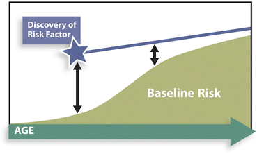

Fig. 1.1
Conceptual representation of diminishing relative risk (RR, ) after discovery of a linear absolute risk, as a result of nonlinear changes in baseline risk
Additional variables can play into declining RRs as well. Note the sharp decline in RRs in the list above associated with mantle radiation in Hodgkin’s disease, starting out at a level comparable to BRCA gene-positivity (RR = 40), declining to no risk at all (RR = 1.0), depending on the “age at exposure” to the radiation. In fact, “age at exposure” has been the major contributor to risk in all radiation-related risk studies with negligible power over the age of 30–40, which should help minimize fears about miniscule radiation exposure with mammography for women over 40.
If one makes the cardinal error of multiplying a relative risk X baseline lifetime risk to arrive at an individual’s lifetime risk, one will quickly see that something is wrong. Using the RR = 40 above, one might be tempted to multiple 40 × “12 %” baseline to arrive at an individualized risk, but this would yield a 480 % probability for breast cancer. The first problem with this approach is what we have already seen with regard to declining RRs over time. Secondly, the “12 %” overstates baseline risk since the “one-in-eight” figure is drawn from general population risk that includes all women with known risk factors in addition to those with no known risks. For women with no known risk factors, lifetime baseline risk is approximately 7 %.
Even if relative risks are accurate and handled with care, problems arise for those patients with more than one risk factor. For instance, in a patient with extreme mammographic density plus a first-degree relative with breast cancer, are these risks additive, synergistic, or overlapping? It may be that the risk imparted by the family history is reflected in the mammographic density, and it would be an error to count the same risk twice. The best way to address this would be through the direct study of risks in pairs. In fact, this has been done, albeit infrequently.
Relative risks when factors are paired: | |
First-degree relative with breast cancer and nulliparity | RR = 2.7 |
First-degree relative with breast cancer and first full-term pregnancy after 30 | RR = 4.0 |
First-degree relative with breast cancer and gross cystic change | RR = 3.0 |
Nulliparity and atypical hyperplasia | RR = 5.0 |
The most familiar pairing of risk factors came from Drs. Page and DuPont in their landmark work with tissue risks, with the finding of synergism between a positive family history and atypical hyperplasia. To confirm this synergism, these investigators included the use of two different denominator populations to validate the relative risk of:
First-degree relative with breast cancer and atypical hyperplasia on biopsy RR = 9.0.
Subsequent studies have not been able to replicate this synergism, however, leaving atypical hyperplasia with a relative risk of 4.0, with or without a positive family history. This translates to substantial differences in absolute risk when these RRs are converted for patient counseling. Thus, one sees support for the argument that risk assessment should deal in generalities and “ranges of risk,” rather than the current trend of mathematical models that carry absolute risk determinations to the right of the decimal point, offering illusory exactitude.
Converting Relative Risks to Absolute Risks
When it became clear that relative risks were a poor way to communicate with patients, several groups began constructing models in the 1980s that would allow clinicians to discuss risk in absolute terms. As it would be impractical to render a final risk assessment based on the direct study of countless combinations of risks as “pairs,” “triplets,” “quadruplets,” etc., the creators of these models had to combine RRs mathematically instead. Although multiplication of RRs is the core principle, the mathematical merger is far more complex. Relative risks based on age (e.g., age at menarche) had to be managed on a “sliding scale” with a reference age serving as “normal.” The contributing RRs are not seen by the user. Only absolute risks are generated. Once the models are created from a data set, then they are confirmed with a different cohort, and ideally, prospectively validated as well.
With absolute risk levels that these models generate, a problem arose immediately with regard to patient counseling—how does the newly calculated risk compare to baseline when there are two distinct baseline references? We have, first of all, a “general population” baseline risk that includes women with risk factors (the well-known “one in eight” or 12 %) and, secondly, the “no risk” baseline of 7 % that is composed of women without any known risk factors.
If one had to pick a single baseline, it would seem that a comparison should be made to the “no-risk” population as this is the approach when RRs are being calculated in the first place. This was tried with one of the more popular models and the feedback was overwhelmingly negative in that outcomes seemed to exaggerate risk. Many women undergoing routine evaluation with minimal apparent risk were deemed “at increased risk.” So, a switch was made to “general population risk,” called “average risk,” which includes the women with known risks. Now, many users of the model are surprised when a patient thought to be “at modest risk” proves to be the same, or below, general population risk.
This confusion over two acceptable definitions of baseline risk has no easy answers. One approach is to use both reference points, comparing the calculated absolute risk in the patient to both a “no risk” baseline and a “general population” baseline, all to provide better perspective.
Absolute Lifetime Risks
Patients and clinicians are most interested in lifetime risks. The first problem here is that we rarely have solid data for lifetime risks. Even the remarkable 55-year follow-up in a cohort of women who received thymic radiation as infants (RR = 3.0) leaves us wondering about the remaining risk for the last 20–40 years of life for these women. With few exceptions, risk calculations are derived from relative risk studies where follow-up is less than “lifetime.” Therefore, lifetime risks tend to be projections.
Then, there are several ways in which lifetime risk can be misstated, either exaggerating or minimizing true risk. As a ground rule, “lifetime” risk for the individual patient implies remaining lifetime risk. Key point: We “pass through” risks as we age, so lifetime cumulative risk might be “one in eight” for an entire life measured from age 0 to 100, but it does not apply to the 60-year-old who has passed through nearly half of that risk already (Fig. 1.2):
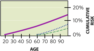

Fig. 1.2
Cumulative lifetime risk for breast cancer is often stated as “1 in 8” or 12 %, but this is total lifetime risk (solid line). Since we pass through risk as we age, remaining lifetime risk diminishes over time. A 60-year-old faces a 7 % baseline remaining lifetime risk (through age 80) for breast cancer when considering “general population” risk (dotted line), and even less (4 %) when considering the “no known risk” population (dashed line)
This concept carries through all strata of risk. For example, it is commonly stated that if a patient tests positive for a BRCA gene mutation, she will be at a 55–85 % risk for the development of breast cancer (as well as high risk for ovarian cancer). This might be true for an “entire lifetime,” but it must be age adjusted for the individual. If the patient is asymptomatic at age 60 when found to harbor a BRCA mutation, her remaining risk for breast cancer is more in the range of 20–30 % over the next 30 years, not 85 %.
It is also possible to underestimate the risk by using short-term studies and not adjusting for patient age. The 30 y/o who is newly diagnosed with lobular carcinoma in situ (LCIS) will learn—either on her own or from other sources—that her risk for invasive breast cancer is “20 %,” a one-size-fits-all number found on multiple Web sites without any reference to risk as a function of time. This “20 %” is a risk elevation that may not seem that much different than the 12 % that all women face, giving the patient a false sense of security. But this 20 % is derived from studies with 20-year follow-up, and all indicators so far point to a 1 %/year risk that extends at least 30 years. More recently, the problem of LCIS risk counseling has worsened, often through third-party payors who, perhaps unwittingly, base their “less than 20 % lifetime risk for LCIS” on studies that had less than 20-year follow-up (at 1 %/year, a 15-year study = 15 % risk). At the other end of the spectrum, a 70-year-old is likely facing only a 10 % remaining lifetime risk for breast cancer after a diagnosis of LCIS, assuming normal life expectancy, compared to a 3–4 % baseline risk. A floating percentage for absolute risk is meaningless outside the framework of time.
(Note for the mathematical purist: If a study reveals 15 % risk over 15 years, admittedly, the yearly risk is not exactly 1 %/year. Each incident case of cancer leaves a smaller pool of unaffected individuals and a slightly different percentage each year, albeit only a very small difference when the total “n” is large. When “%/year” data is offered in this chapter, it is meant only as a close estimate used to counsel patients.)
Regarding these long-term calculations for risk, the mathematical models below will automatically calculate remaining lifetime cumulative risk over a defined period of time, thus preventing the error of quoting a “total” lifetime risk. However, nothing can overcome this paradox: As a patient ages, her remaining lifetime risk is declining, while her short-term incidence for breast cancer is rising and peaking (Fig. 1.3).
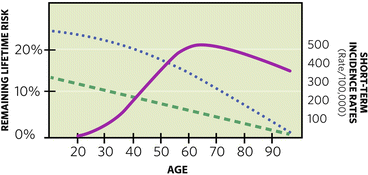

Fig. 1.3
Instead of the rising curve of cumulative lifetime risk, “remaining” lifetime risk in the general population declines as noted by the dashed line, while a “high risk” curve declines as noted by the dotted line. For illustrative purposes, 5-year incidence rates, smoothed to a solid-line curve, are overlaid to approximate short-term probabilities for breast cancer that are rising through age 60
This paradox will lead to some improbable management guidelines when it comes to interventions, some based on short-term calculations, while others based on “lifetime” risks. But first, a look at the more commonly used mathematical models.
The Mathematical Models
In the 1980s, with the prospect of tamoxifen as a risk-reducing agent, the need arose for a mathematical model that would standardize risk assessment, allowing an objective entry threshold to a large-scale clinical trial, as well as serving to calculate the size of the trial necessary for statistical significance.
The Gail Model (later modified to the National Cancer Institute Breast Cancer Risk Assessment Tool, or Gail 2) was adopted for the NSABP P-01 trial that randomized patients to receive either tamoxifen or placebo. The threshold for entry was a Gail-calculated 5-year absolute risk of 1.67 % or greater, a risk level achieved simply by being age 60. While this confused many (How can a “normal risk” 60 y/o be labeled “high risk?”), the NSABP was dealing with the aforementioned paradox of peak short-term incidence vs. declining lifetime risk. In supporting this approach, it should be noted that clinical trial design mandates the greatest amount of information in the shortest time possible, so the initial focus needed to be on short-term risk and short-term outcomes.
Importantly, the trial not only proved the efficacy of reducing breast cancer risk with tamoxifen but also prospectively validated the Gail model as a tool to assess breast cancer risk. This validation came through comparing the number of predicted (expected) cancers for the control group versus those actually observed. The Gail model, derived from data generated by the Breast Cancer Detection and Demonstration Project (BCDDP), was also validated when applied to well-known studies such as the Cancer and Steroid Hormone Study (CASH), and the Nurses’ Health Study (NHS). In 1999, the Gail model was modified to Gail 2 or NCI-Gail using age-specific incidence rates obtained from the Surveillance, Epidemiology, and End Results (SEER) database.
A proliferation of proposed models followed with varying degrees of validation. Clinicians do not necessarily need to know the details of each model, with regard to the internal relative risks at work; however, some degree of familiarity with the models, including strengths and weaknesses, is important given our dependence on these models for current interventional guidelines.
Risk assessment programs at breast screening centers and cancer centers have proliferated along with the models, and the skill in risk analysis comes not through simple data entry into the models, but through understanding which models are most appropriate for a given patient. It is equally important for the practitioner of risk assessment to develop the skill of estimating risks without models such that errors in data entry can be recognized, rather than blindly transmitting misleading risk information to patients who are making serious decisions about interventions.
Brief summaries of the breast cancer risk assessment models are listed below:
Gail-NCI model (download at http://www.cancer.gov/bcrisktool/): This model is the easiest to use and the most thoroughly validated for predicting the risk of invasive cancer. Note a distinction here that other models, including the first version of the Gail model, calculate the risk for both invasive disease and DCIS. Gail-NCI incorporates reproductive/endocrine risks, family history, and tissue risks. However, it has a number of caveats: family history is limited to first-degree relatives with breast cancer; there is no provision for the ages of these relatives when diagnosed, nor is there a provision for family members with ovarian cancer. Thus, the model carries the disclaimer that it is inappropriate to use the Gail model if one suspects a BRCA gene mutation. Also, there is no provision for assessing the risk of LCIS. The model conveniently calculates 5-year absolute risks or lifetime risks or anything in between. There have been efforts all along to improve the model, and more emphasis is now being paid to ethnicity. The model can overestimate the risk if a patient has had a large number of benign breast biopsies in the past. And, some experts believe it can underestimate the risk for women with atypical hyperplasia where histology has been confirmed by expert pathology review. Finally, a rarely discussed weakness is the fact that the Gail model does not include the number of women in the family without breast cancer, information that can reveal truncated family histories wherein breast cancer risk and BRCA mutation probabilities might be understated.
Stay updated, free articles. Join our Telegram channel

Full access? Get Clinical Tree


