Radiation Therapy Using High-Energy Electron Beams
Bruce J. Gerbi
Introduction
High-energy electrons have been commonly available in radiation therapy for the treatment of cancer since the early 1950s and their availability in modern radiation therapy departments is simply expected. The most useful electron energies in clinical settings range from 6 to 20 MeV with the intermediate beam energies being the most clinically useful. Electrons are used for specific purposes within a radiation therapy department mainly due to their precise depth of penetration and ability to deliver a high dose to the superficial regions of the body. They are most useful for treatments of the skin, scars, chest wall treatments post-mastectomy, and for superficial nodal treatments. They are also particularly well suited for treatments of targets that lie above sensitive structures such as the spinal cord, lung, or heart.
The energy of a clinical beam is described by the most probable energy at the surface at the standard treatment distance (usually 100 cm source–skin distance [SSD]) and represents the energy possessed by the majority of the incident electrons at that location. Thus, when a particular electron energy is selected for use on a linear accelerator, this is the closest integer value to the actual energy of the electron beam hitting the patient’s surface.
High-Energy Electron Characteristics
Electrons are directly ionizing particles that possess a negative charge and are low in mass compared to protons and neutrons. As charged particles, they interact directly with the absorbing material, being attracted to positive charges and repelled by negative charges. These forces of attraction or repulsion are called Coulomb interactions and result directly in ionizations and excitations within the absorbing medium. Because the mass of an electron is ∼1/2,000 of the mass of protons and neutrons, its direction of travel can be easily changed by interactions with these more massive particles. Thus, electrons are easily scattered by the absorbing medium. As electrons pass through a material, their average energy decreases due to either collisions or radiative processes until they are eventually captured by the atoms of the absorbing material. It is the location at which these electrons scatter, where bonds are broken, and where ionization and excitation take place that dictates where radiation dose is deposited within a medium, or more importantly, within patients.
Change in Central Axis Percentage Depth-Dose with Change in Beam Energy
The central axis (CA) percentage depth-dose curve is a display of the dose at depth along the CA of the beam compared to the dose at the depth of maximum dose. The CA percentage depth-dose characteristics of electron beams are fundamentally dependent upon the types of interactions that incident high-energy electrons undergo, as described above. From a clinical standpoint, the shape of the CA percentage depth-dose curve for an electron beam depends most notably on beam energy, field size, the angle of beam incidence, collimation, and SSD. Figure 19.1 shows typical CA percentage depth-dose curves in water for 10 × 10 cm2 electron beams from a Varian 2300CD linear accelerator. The plot shows beam energies for 6, 9, 12, 15, 18, and 22 MeV electrons. As can be seen in the figure, the dose at the surface for electron beams is much higher than what is exhibited by photon beams. The surface dose (which is the dose in the first 0.05 cm) is ∼75% for 6 MeV electrons increasing with energy to over 90% at the surface for the 22 MeV electron beam. This increase in surface dose with increasing beam energy occurs because lower energy electrons are scattered more easily and through larger angles than are electron beams of higher energy. This causes the dose to increase more rapidly and over shorter distances for low-energy electron beams at the surface. As electrons penetrate more deeply into the medium, the depth of maximum dose is reached. Contrary to megavoltage photon beams, the depth at which the maximum dose occurs for electron beams does not follow a specific trend of increasing with increasing beam energy. The depth of maximum dose is also dependent on linear accelerator design and the accessories used for the treatment. Beyond the depth of dmax, higher energy electrons penetrate more deeply and falloff less rapidly per centimeter than lower energy electrons. At depths greater than the practical range, Rp, the CA electron percentage depth-dose curve decreases slowly with depth since the dose in this region is contributed mainly by straggling electrons and bremsstrahlung radiation. The practical
range of the beam is defined as the depth at which the straight line decreasing portion of the electron CA percentage depth-dose curve intersects a line describing the photon contamination of the beam. A good estimate of the practical range of the beam in centimeters can be obtained by taking the energy of the beam, in MeV, and dividing it by 2. An Rp of 11 cm is shown in Figure 19.1 for the 22 MeV electron beam. The photon contamination is ∼1% for 6 MeV rising to approximately 6% to 7% for the 22 MeV beam. This photon contamination is the result of electron interactions with the exit window of the linac, the scattering foils, the beam ion-chamber, the collimator jaws, or treatment apparatus. Additional x-rays can also be produced within the patient, although the magnitude of this contribution is not very large.
range of the beam is defined as the depth at which the straight line decreasing portion of the electron CA percentage depth-dose curve intersects a line describing the photon contamination of the beam. A good estimate of the practical range of the beam in centimeters can be obtained by taking the energy of the beam, in MeV, and dividing it by 2. An Rp of 11 cm is shown in Figure 19.1 for the 22 MeV electron beam. The photon contamination is ∼1% for 6 MeV rising to approximately 6% to 7% for the 22 MeV beam. This photon contamination is the result of electron interactions with the exit window of the linac, the scattering foils, the beam ion-chamber, the collimator jaws, or treatment apparatus. Additional x-rays can also be produced within the patient, although the magnitude of this contribution is not very large.
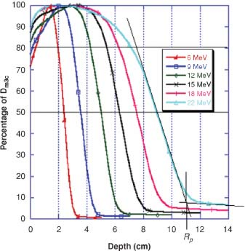 Figure 19.1. Electron central axis percentage depth-dose curves for a Varian 2300CD, 10 × 10 cm2 cone, 100 cm SSD. |
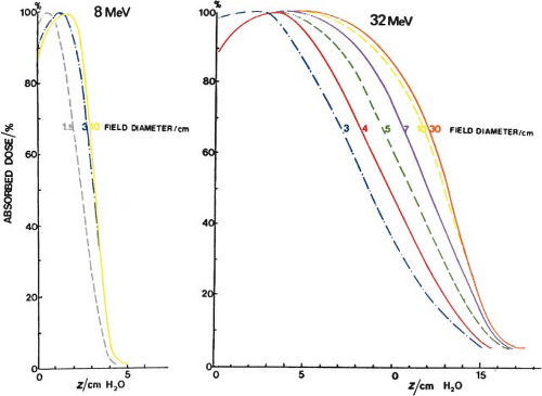 Figure 19.2. The change in percentage depth dose for high-energy electrons with change in field size. Source: From ICRU. International commission on radiation units and measurements, radiation dolsimetry: electron beams with energies between 1 and 50 MeV, ICRU Report 35. Bethesda, MD: International Commission on Radiation Units and Measurement, 1984. |
Change in Central Axis Percentage Depth Dose with Change in Field Size
Standard electron cone sizes for linear accelerators typically range from 6 × 6 to 25 × 25 cm2. There is significant change in CA percentage depth dose with field size when the field size decreases to less than the practical range for that electron beam energy. This is because of the loss of side scatter with decreasing field size, and is shown by the data in Figure 19.2. There is a shift in both the depth of dose maximum and the D90 dose toward the surface with decreasing field size but the Rp is unchanged. Clinical data for an Elekta Synergy linear accelerator is shown in Table 19.1. For the 6 MeV beam data, the CA percentage depth dose is the same for all field sizes within the measurement accuracy of the data. For the more energetic 18 MeV beam, the CA percentage depth dose is slightly less for the 6 × 6 cm2
cone size as compared to the two larger cone sizes since the practical range of the 18 MeV beam is ∼9 cm. The data in the build-up region were taken using an Attix plane–parallel ionization chamber in a solid water phantom while the data deeper than the dmax point was taken using a Therados electron diode.
cone size as compared to the two larger cone sizes since the practical range of the 18 MeV beam is ∼9 cm. The data in the build-up region were taken using an Attix plane–parallel ionization chamber in a solid water phantom while the data deeper than the dmax point was taken using a Therados electron diode.
Table 19.1 Central Axis Percentage Depth Doses for 6 and 18 MeV Electrons from an Elekta Synergy Linear Accelerator | ||||||||||||||||||||||||||||||||||||||||||||||||||||||||||||||||||||||||||||||||||||||||||||||||||||||||||||||||||||||||||||||||||||||||||||||||||||||||||||||||
|---|---|---|---|---|---|---|---|---|---|---|---|---|---|---|---|---|---|---|---|---|---|---|---|---|---|---|---|---|---|---|---|---|---|---|---|---|---|---|---|---|---|---|---|---|---|---|---|---|---|---|---|---|---|---|---|---|---|---|---|---|---|---|---|---|---|---|---|---|---|---|---|---|---|---|---|---|---|---|---|---|---|---|---|---|---|---|---|---|---|---|---|---|---|---|---|---|---|---|---|---|---|---|---|---|---|---|---|---|---|---|---|---|---|---|---|---|---|---|---|---|---|---|---|---|---|---|---|---|---|---|---|---|---|---|---|---|---|---|---|---|---|---|---|---|---|---|---|---|---|---|---|---|---|---|---|---|---|---|---|---|
| ||||||||||||||||||||||||||||||||||||||||||||||||||||||||||||||||||||||||||||||||||||||||||||||||||||||||||||||||||||||||||||||||||||||||||||||||||||||||||||||||
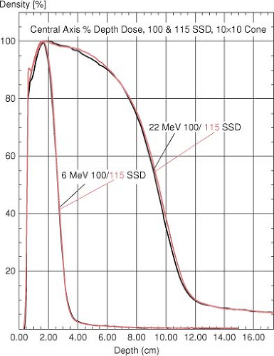 Figure 19.3. Central axis percentage depth-dose curve for 100 and 115 cm SSD. The slight difference in central axis percentage depth dose observed for the 22 MeV beam is due to field size differences rather than SSD effects. |
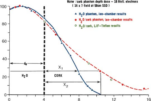 Figure 19.4. Depth-dose distribution in water and water-cork phantoms. Source: Modified from Almond P, Wright A, Boone M. High-energy electron dose perturbations in regions of tissue heterogeneity. Radiology 1967;88: 1146. |
Change in Central Axis Percentage Depth Dose with Change in SSD
There is only a slight change in the CA percentage depth-dose values at extended treatment distances. In the buildup region of the curve, the difference between the 100 and 115 cm SSD data is clinically insignificant (Fig. 19.3). At depths deeper than the location of dmax, no difference is observed in the 100 cm SSD curve versus the 115 cm SSD data. For the 20 MeV data, the 80% to 95% isodose lines beyond the depth of the dmax show very slight but clinically insignificant differences between the 100 and the 115 cm SSD curves. This is because the 10 × 10 cm2 field at 100 cm diverges to an 11.5 × 11.5 cm2 field at 115 cm SSD.
Change in Central Axis Percentage Depth Dose due to Inhomogeneities
The CA percentage depth-dose curve can be significantly changed from those measured in water by the presence of non-unit density inhomogeneities such as lung, bone, air cavities, or other non-unit density materials. For small inhomogeneous regions, it is difficult to calculate accurately the dose distribution because of the complicated nature of the scatter in and around these areas. For larger regions of inhomogeneous material, the amount of change in the CA percentage depth-dose curve depends on the electron density of the material compared to the electron density of water. For lung tissue and air cavities whose electron density is lower than that of water, the electrons penetrate to a deeper depth than they would in a water medium. This change in the depth of penetration is shown in Figure 19.4 using cork to represent lung tissue. For compact bone whose electron density is greater than water, a proportionate decrease in the depth of penetration of the electrons is seen.
Two- and Three-Dimensional Dose Distributions for Electron Beams
Off-Axis Beam Characteristics: Flatness and Symmetry
A uniform intensity across the electron-beam field is a requirement for clinical use of high-energy electrons in radiation therapy. As with photon beams, the off-axis ratio (OAR) relates the dose at any point in a plane perpendicular to the CA of the beam to the dose at the CA of the beam. A plot of the OAR versus distance from the CA is called a dose profile (Fig. 19.5). According to the AAPM Task Group 25 report, both symmetry and flatness should be verified on each of the principle and diagonal axis of the beam for the largest field for each applicator. Flatness specifications should be checked at several collimator and gantry angles. The reference plane is defined in TG-25 report “as a plane, parallel to the surface of the phantom and perpendicular to the CA of the beam at the depth of the 95% isodose beyond the depth of dose maximum.” “The flatness of the bean normalized to the CA should not exceed ±5% (optimally within ±3%) over an area within lines 2 cm inside the geometric edge of fields that are equal to or larger than 10 × 10 cm2.” The symmetry of the beam in the reference plane should not differ by >2% at any pair of points symmetrically located at an equal distance from the CA of the beam. These measurements of flatness and symmetry should be done at the time of linac installation and should be verified monthly and following any major service of the linear accelerator (1,2,3).
Isodose Curves for Normal Beam Incidence
Isodose curves are a collection of lines that join points of equal dose that show the variation in dose as a function of depth and distance away from the CA. The depth-dose data for fixed SSD beams are normalized to the point of maximum dose on the CA of the beam and are drawn at 10% intervals. Figure 19.6 shows typical isodose curves for electron beams (6 and 22 MeV) for a 10 × 10 cm2 field from a Varian 2300CD accelerator. Isodose curves for electron beams are dependent on the beam energy, field size, collimation, and SSD. The 50% isodose curve almost follows beam divergence from the surface while the 90% and 80% isodose curves are pinched in toward the CA of the beam. Isodose curves lower than 50%, bow out, away from the CA, producing the distinctive isodose curve shape for high-energy electron beams. In clinical situations, the field size should be larger than the borders of the target by at least 1 cm to ensure that it is adequately covered by the 90% isodose line.
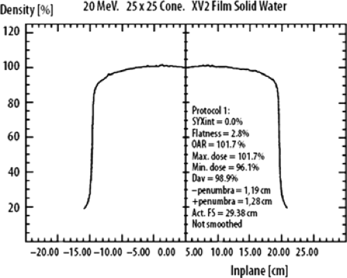 Figure 19.5. Flatness and symmetry plot for a 20 MeV, 25 × 25 cm2 electron cone. The data is derived from an irradiated piece of Kodak XV2 film placed at the depth of maximum for the beam and scanned using a Wellhofer film scanner using WP700 software. Source: From Gerbi BJ. Clinical applications of high-energy electrons. In: Levitt SH, Purdy JA, Perez CA, et al., eds. Technical basis of radiation therapy: practical clinical applications, 4th ed. Berlin: Springer, 2006; Figure 7–6. |
Isodose Distributions at Extended Treatment Distances
Figure 19.7 shows 9 and 20 MeV electron isodose curves at 100 and 115 cm SSD illustrating the influence of increasing the treatment distance on the shape of the isodose curves incident on a flat phantom. Because of the increased distance from the end of the electron cone, electrons scatter out of the beam resulting in a loss of sharpness in the edge of the beam both outside the 50% isodose line and inside the 50% line. The loss of field sharpness has critical clinical importance in both matching electron fields at extended distances and when choosing field sizes to cover the target region.
The final shape of the isodose curves can be influenced by factors such as patient curvature, inhomogeneities such as lung, bone, high-Z materials, and field-shaping devices such as cerrobend inserts, lead cutouts that are placed on the patient’s skin surface, and internal shields designed to protect sensitive or normal tissues.
Isodose Distributions for Curved and Irregular Surfaces
Radiation fields are seldom incidents on flat surfaces. The more common situation is that the beam is incident on a curved surface, surfaces with multiple changes in contour, or on oblique surfaces. This is clearly evident in treatments of the post-mastectomy chest wall, extremities, the scalp, areas in and around the eyes, nose, or ears, or where complex skin folds are involved. Surgical areas can also create abrupt changes and irregularities in the patient’s surface. Treatments of any of these areas of the body dramatically change the isodose characteristics of electron beams from what is measured for normally incident electron beams on flat surfaces. Figure 19.8 shows isodose
curves for an electron beam incidents on a curved surface such as a post-mastectomy chest wall. The isodose curves follow roughly the curvature of the external contour but there are other changes due to attenuation of the beam, obliquity effects, loss of scatter, and decrease in the beam intensity due to inverse square decrease with increased distance from the end of the electron applicator. As the angle of beam incidence becomes more oblique, the maximum dose moves more toward the surface, and the shape of the CA percentage depth-dose curve changes dramatically, but the depth of maximum penetration of the beam stays essentially the same. Table 19.2 from Khan (4), shows numerically the change in the CA percentage depth dose as a function of the angle of electron beam incidence for various electron energies for angles of incidence of 30, 45, and 60 degrees.
curves for an electron beam incidents on a curved surface such as a post-mastectomy chest wall. The isodose curves follow roughly the curvature of the external contour but there are other changes due to attenuation of the beam, obliquity effects, loss of scatter, and decrease in the beam intensity due to inverse square decrease with increased distance from the end of the electron applicator. As the angle of beam incidence becomes more oblique, the maximum dose moves more toward the surface, and the shape of the CA percentage depth-dose curve changes dramatically, but the depth of maximum penetration of the beam stays essentially the same. Table 19.2 from Khan (4), shows numerically the change in the CA percentage depth dose as a function of the angle of electron beam incidence for various electron energies for angles of incidence of 30, 45, and 60 degrees.
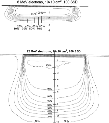 Figure 19.6. Typical 6 and 22 MeV electron curves, 10 × 10 cm2 electron cone, 100 SSD, Varian 2300CD. The data was taken using Kodak XV2 film placed parallel to the incident beam in a solid water phantom and scanned using a Wellhofer film scanner using WP700 software. |
Isodose Distributions Involving Inhomogeneities
High-energy electrons are greatly affected by the presence of inhomogeneities in the body. The effects of the presence of bone, lung, air, teeth, and implanted materials greatly influence the scattering and interactions of electrons and consequently the final distribution of dose within the body. Electron depth-dose distributions are dependent on the electron density of the materials through which the beam passes and ultimately on the physical density of these materials. Because lung is one-fourth to one-third the density of normal tissue (5), high-energy electrons travel three to four times farther in this material than in unit density material. When using electrons for treatment of the post-mastectomy chest wall, the desire is to put the 80% isodose line at the lung chest-wall interface. This adequately treats the tissues of the chest wall but can lead to a high dose to the underlying lung. Figure 19.9 illustrates the challenges associated with the use of electrons in this region and shows the enhanced penetration in lung as compared to normal tissue. Bolus is often used to ensure not only that the 80% isodose line lies at the chest wall–lung interface, but also that a high dose is given to the skin surface.
Bones are often present in the treatment region when using electrons. Bone density can vary in density from approximately 1.0 to 1.1 g/cm3 for spongy bone to 1.5 to 1.8 g/cm3 for compact bone found in the skull, mandible, or the long bones that provide strength and support in the body. The ribs are also quite important to consider when
treating the chest wall. Figure 19.10 shows the difference in the shape of the isodose distribution of 17 MeV electrons when a slab of bone is present in the beam as compared to the isodose distribution produced in a unit density phantom. With the bone present, the electron isodose curves are shifted toward the surface because of the extra attenuation in bone. In addition, the dose is increased at the edges of the bone due to the enhanced scattering of electrons into this region. Underneath the bone edge, there is an area of decreased dose due to the loss of side scatter equilibrium.
treating the chest wall. Figure 19.10 shows the difference in the shape of the isodose distribution of 17 MeV electrons when a slab of bone is present in the beam as compared to the isodose distribution produced in a unit density phantom. With the bone present, the electron isodose curves are shifted toward the surface because of the extra attenuation in bone. In addition, the dose is increased at the edges of the bone due to the enhanced scattering of electrons into this region. Underneath the bone edge, there is an area of decreased dose due to the loss of side scatter equilibrium.
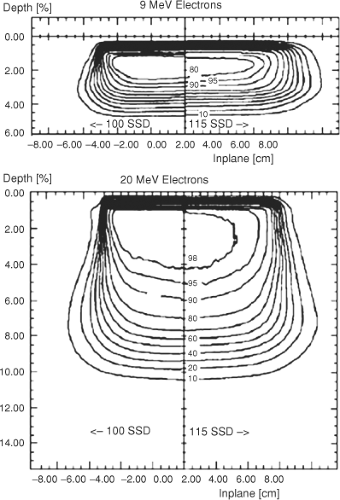 Figure 19.7. Electron isodose curves for 9 and 22 MeV electrons at 100 and 115 cm SSD produced with a 10 × 10 cm2 cone. |
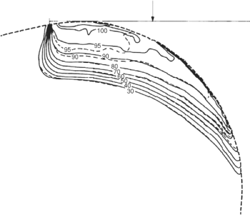 Figure 19.8. Electrons incident on a curved surface. |
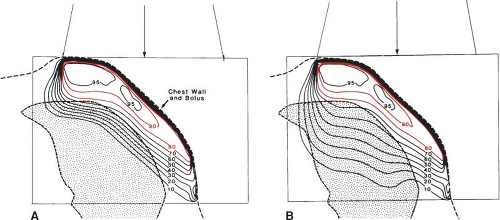 Figure 19.9. An example of chest wall irradiation using 13 × 15 cm2, 10 MeV electrons (effective SSD = 68 cm) showing enhanced penetration into lung. A: Calculated isodose curves uncorrected for lung density. B: Calculated isodose curves corrected for lung density (ρ = 0.25 g/cm3). Bolus was added to the surface to even out chest wall thickness and maximize the surface dose. |
The presence of air cavities (ρ = 0.0013 g/cm3) in the path of electron beams has a large effect on the final distribution of electrons within the body. Because of complicated scattering at the tissue–air interfaces, a significant reduction in dose to the tissues adjacent to the air cavity can lead to underdosing of 10% or more (6). This could result in an inadequate dose being delivered to the target region. Figure 19.11 (6) shows the electron distribution for treatments in the nasal region when both bone and air cavities are taken into account. In comparison to an electron dose distribution, which assumes the region to be
unit density, a much higher dose to the brain stem, brain, and underlying anatomy is actually delivered than what would be expected if only unit density materials were used in the calculation.
unit density, a much higher dose to the brain stem, brain, and underlying anatomy is actually delivered than what would be expected if only unit density materials were used in the calculation.
| |||||||||||||||||||||||||||||||||||||||||||||||||||||||||||||||||||||||||||||||||||||||||||||||||||||||||||||||||||||||||||||||||||||||||||||||||||||||||||||||||||||||||||||||||||||||||||||||||||||||||||||||||||||||||||||||||||||||||||||||||||||||||||||||||||||||||||||||||||||||
 Compared with that at Normal Beam Incidence (
 = 0 degree)
 = 30 degrees
 = 45 degrees
 = 60 degrees
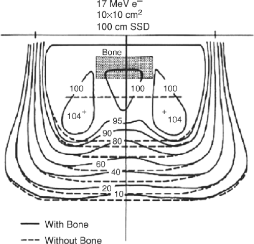 Figure 19.10. The effect of compact bone on 17 MeV electron isodose curves. Source: From Hogstron K. Dosimetry of electron heterogeneities. In: Wright A, Boyer A, eds. Advances in radiation therapy treatment planning. New York, NY: American Institute of Physics, Inc., 1983:223–243. |
High-Z materials can also be present in electron beams in the form of implanted prosthetic devices (7), fillings for dental cavities, or deliberately as internal shields designed and used to limit the dose to underlying tissue. Implanted devices and materials most commonly consist of advanced polymers, ceramic materials, stainless steel, and titanium. Internal shields are fabricated from several materials and can consist of aluminum, lead, tungsten, and gold or a combination of these materials. The classic graph of electron backscatter versus atomic number, Z (Fig. 19.12) (8)
shows the relative amount of backscatter observed from different atomic number materials as a function of electron beam energy at the interface. This shows that there is increased backscatter with increasing Z and decreasing energy of the electrons at the interface. Figure 19.13 shows the intensity of the backscattered electrons from lead transmitted through polystyrene in the upstream direction of the incident electron beam (9). Whether designing internal shields for the protection of underlying material or when dealing with implanted materials used from the treatment of other medical conditions, the effects of these high-Z materials on the final dose distribution must be carefully evaluated.
shows the relative amount of backscatter observed from different atomic number materials as a function of electron beam energy at the interface. This shows that there is increased backscatter with increasing Z and decreasing energy of the electrons at the interface. Figure 19.13 shows the intensity of the backscattered electrons from lead transmitted through polystyrene in the upstream direction of the incident electron beam (9). Whether designing internal shields for the protection of underlying material or when dealing with implanted materials used from the treatment of other medical conditions, the effects of these high-Z materials on the final dose distribution must be carefully evaluated.
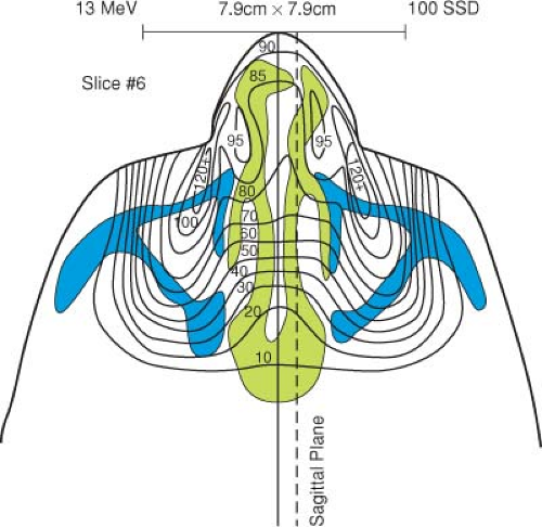 Figure 19.11. The effect of the abrupt change in surface contour by the nose and the effect on the final isodose distribution. The plan is done assuming unit density material and not taking into account the air cavities in this region of the body. Source: From Chobe R, McNeese M, Weber R, et al. Radiation therapy for carcinoma of the nasal vestibule. Otolaryngol Head Neck Surg 1988;98:67–71. |
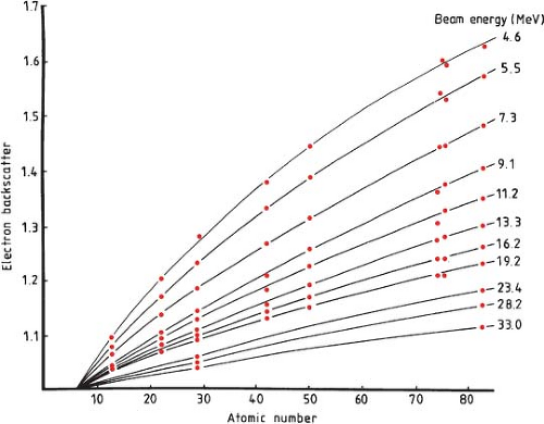 Figure 19.12. The relative amount of electron backscatter for various electron beam energies above different atomic number materials. Source: From Klevenhagen SC, Lambert GD, Arbabi A. Backscattering in electron beam therapy for energies between 3 and 35 MeV. Phys Med Biol 1982;27:363–373. |
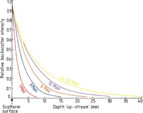 Figure 19.13. The intensity of backscatter from lead through polystyrene for different electron beam energies. Source: From Lambert G, Klevenhagen S. Penetration of backscattered electrons in polystyrene for energies between 1–25 MeV. Phys Med Biol 1982;27:721. |
Clinical Use of Electron Beams
Dose Prescription—ICRU 71
Report 71 of the International Commission on Radiation Units and Measurements (ICRU) was published in 2004. This report described new recommendations for “prescribing, recording, and reporting electron beam therapy” (10). They recommended that the same dose prescription approach be used for electron treatments as for photons as specified in ICRU Reports 50 and 62 for photon beams (11,12). The concepts of gross tumor volume (GTV), clinical target volume (CTV), planning target volume (PTV), treated volume, organs at risk, and planning organ at risk volume (PRV) were defined as for photon beam treatment planning purposes. The treatment was to be specified completely, including time-dose characteristics making no adjustments in the relative biological effectiveness differences between photons and electrons. For reporting electron doses, they recommended the selection of a reference point referred to as the “ICRU reference point.” This point should always be chosen at the center (or central part) of the PTV and should be clearly described. In general, the beam energy is selected so that the maximum of the depth-dose curve on the beam axis is located at the center of the PTV. If the peak dose does not fall in the center of the PTV, then the ICRU reference point for reporting should be selected at the center of the PTV and the maximum dose should also be reported. For reference electron irradiation conditions, they also recommend that the following dose values be reported (10):
The maximum absorbed dose to water.
The location of and dose value at the ICRU reference point if not located at the level of the peak absorbed dose.
The maximum and minimum doses in the PTV, and dose(s) to OARs derived from dose distributions and/or dose–volume histograms. For small and irregularly shaped beams, the peak absorbed dose to water for reference conditions should be reported. It is also recommended that when corrections for oblique incidence and inhomogeneous material are applied, the application of these corrections should be reported.
Dose reporting guidelines for the special techniques of intraoperative radiation therapy (13) and total skin irradiation (TSI) are also provided in ICRU Report 71. The treatment goal for TSI is to deliver a uniform dose to the total skin surface. For patients with superficial disease, TSI can be delivered with one electron energy. However, the thickness of the skin disease may vary with stage, pathology, and location on the body surface. For such cases, several CTVs need to be identified and different electron beam energies may be required to treat the various regions. For each anatomical site, an ICRU reference point at or near the center of the PTVs/CTVs has to be selected for reporting. The reference point may be at the level of the peak dose if it is located in the central part of the PTV. In addition, an ICRU reference point that is clinically relevant and located within the PTV can be used for the entire PTV.
ICRU Report 71 recommended the reporting of the following dose values:
The peak absorbed dose in water for each individual electron beam
The location of and dose value at the ICRU reference point for each anatomical area
The best estimate of maximum and minimum dose to each anatomical area
The location and absorbed dose at the ICRU point for the whole PTV, and best estimate of the maximum and minimum doses for the whole PTV
Any other dose value considered as clinically significant
IORT is used after surgical intervention to deliver a large single-fraction dose of high-energy electrons to a well-defined anatomical location. ICRU Report 71 recommends
that all devices that are used for IORT need to be reported. This includes the IORT applicator system specifying type, shape, bevel angle, and size of the applicator. The ICRU reference point for reporting is always selected in the center or central part of the PTV, and at the level of the maximum dose on the beam axis, when possible.
that all devices that are used for IORT need to be reported. This includes the IORT applicator system specifying type, shape, bevel angle, and size of the applicator. The ICRU reference point for reporting is always selected in the center or central part of the PTV, and at the level of the maximum dose on the beam axis, when possible.
The ICRU recommended that the following dose values be reported for IORT (10):
The peak absorbed dose to water, under reference conditions, for each individual beam (if the beam axis is perpendicular to the tissue surface).
The maximum absorbed dose in water on the “clinical axis” for oblique beam.
The location of and dose value at the ICRU reference point (if different from above).
The best estimate of the maximum and minimum doses to the PTV. Usually, the irradiation conditions (electron energy, field size, etc.) are selected so that at least 90% of the dose at the ICRU reference point will be delivered to the entire PTV.
Output Determination
For clinical treatments, the determination of dose per monitor unit for each electron treatment is critical. The first step in this determination is the proper calibration of each electron beam energy according to an accepted calibration protocol. The AAPM Task Group 51 report (14) describes in detail the steps that need to be taken to determine the dose rate in terms of gray (Gy) per monitor unit (U) at a reference point in an electron beam for a specified field size and treatment distance. The IAEA TRS Report 398 was developed in parallel with AAPM TG-51 and is very similar in its calibration approach (15). Both calibration protocols use a dose to water calibration factor. For these calibration protocols, the dose rate in water is determined at the depth of dref at 100 cm SSD along the central axis of the electron beam. The calibration field size is 10 × 10 cm2 unless the R50, the depth of the 50% isodose line, is >8.5 cm. A 20 × 20 cm2 field or larger is to be used for these higher beam energies. The calibration is to be performed at the depth of dref, which is defined as 0.6 R50 – 0.1 cm. The depth of dref is close to the depth of dmax for electron energies below about 12 MeV but is deeper than dmax for electron beams of higher energy. This is important to note since the electron CA percentage depth-dose curves are all normalized to the depth of dmax.
The output for each electron beam energy of a linac for a 10 × 10 cm2 cone is set to deliver 1.0 cGy per monitor unit at the depth of dmax. The output for every other electron cone is expressed as a ratio of the output of the 10 × 10 cm2 cone. Thus, if the measured output at dmax for a 15 × 15 cm2 cone when operated at 6 MeV is 1.008 cGy per monitor unit, then the 15 × 15 cm2 electron cone factor would be 1.008 cGy/U divided by 1.000 cGy/U equaling a cone factor of 1.008. A general expression for the output factor from AAPM Report 99 from Task Group 70 is, … the output factor Se for a particular electron field size ra at any treatment SSDra is defined as the ratio of the dose per monitor unit, D/U (Gy/MU), on the central axis at the depth of maximum dose for that field, dmax(ra), to the dose per monitor unit for the reference applicator, or field size r0, and standard SSDr0 at the depth of maximum dose for the reference field used in calibration, dmax(r0). In equation form:
Output Determination: Blocked/Restricted Fields
When electron treatment fields are small, irregular in shape, or both, or when the field is smaller than or close to the minimum radius required for lateral scatter equilibrium, the depth of maximum dose moves toward the surface, the central axis percentage depth dose decreases, and the output decreases as compared to the unrestricted field. This minimum radius, Req, has been shown (17) to be well represented by the equation
where Req is in centimeters and Ep,0 is expressed in MeV. Ep,0 is the most probable energy at the phantom surface (18) and is given by the equation
for water with the practical range, Rp, given in centimeters. Either custom measurements should be performed or analytical approaches described in the historical literature should be done for electron fields whose size is below this minimum radius. Alternatively, a collection of measured outputs for various irregularly shaped fields can be assembled against which a new irregularly shaped field can be compared. Actual measurements of dose rate, depth dose, and isodose distributions can be performed with ionization chambers, diodes, or various films but film can be the most efficient detector to quickly capture this information. A single film in a water equivalent solid phantom can be irradiated parallel to the electron beam with the patient cutout in place and used to determine the depth of dmax for the restricted field. This film can then be used to indicate the shape of the isodose curves for the field in that measurement plane to help assess if the electron field adequately covers the target to be treated. Once the dmax for the restricted field is determined from this first film, a second piece of film can be irradiated perpendicular to the incident electron beam at this depth in a water equivalent solid phantom with the cutout in place. The optical density on this film can be compared to a third film placed
perpendicular to the beam at the depth of dmax for the unrestricted field and irradiated with the 10 × 10 cm2 cone in place. By comparing the optical density of the 10 × 10 cm2 film with that of the optical density of the film for the restricted field, the output in terms of dose per monitor unit for the restricted field can be determined. In addition, the isodose curves for the restricted field can be well described by the data represented on the two films taken with the restricted field cutout in place using automated film scanning software.
perpendicular to the beam at the depth of dmax for the unrestricted field and irradiated with the 10 × 10 cm2 cone in place. By comparing the optical density of the 10 × 10 cm2 film with that of the optical density of the film for the restricted field, the output in terms of dose per monitor unit for the restricted field can be determined. In addition, the isodose curves for the restricted field can be well described by the data represented on the two films taken with the restricted field cutout in place using automated film scanning software.
Small and irregular electron fields can be assessed using verified computational techniques (17,19,20,21,22,23,24) in place of direct measurements. Several analytical approaches are available in the historic literature that describe how to determine output, the shift in dmax, and the central axis percentage depth dose values for restricted fields. The CA depth-dose values for a rectangular electron field whose sides measure X and Y can be determined by taking the square root of the product of the depth doses for the square fields whose sides are X and Y (25) as shown by the equation:
Related posts:

Stay updated, free articles. Join our Telegram channel

Full access? Get Clinical Tree


