Proton Beam Therapy
Hanne M. Kooy
Judy A. Adams
Introduction
Proton beam radiotherapy further advances a central aim of radiation therapy: significant reduction in healthy tissue dose and, as a corollary, significant safe increase in malignant tissue dose. Proton beam radiotherapy is not new and was used as a definitive modality as early as 50 years ago. Its recent emergence as a viable, and even necessary, technology is a consequence of its historical success in treating otherwise incurable disease, the present desire for increased conformal radiation therapy, and the commercial availability of proton beam equipment.
The evolution of proton and photon radiotherapy is diametrically opposite. Proton radiotherapy was, ab initio, a conformal modality but only sparsely available; radiotherapy was a therapeutic analog to planar x-ray imaging and broadly available. Of course, brachytherapy also was, and is, a local conformal modality but has its own application and is in equal competition to proton and photon radiotherapy.
Proton radiotherapy from its inception required careful attention to detail as a consequence of the intrinsic precision afforded by the proton beam itself even while the supporting technologies were minimal. As a result, the early adopters of proton beam radiotherapy were neurosurgeons: Dr. Lars Leksell in Stockholm, Sweden and Dr. Raymond Kjellberg in Boston, USA. Neurosurgeons, by training, have an exquisite understanding of the cranial anatomy as visualized on x-rays, as CT was not yet available. The early use was in abnormalities visible on those x-rays such as pituitary and arterio-venous abnormalities. The x-ray information allowed effective use of the advantageous properties of the proton beam. Easy access to a proton beam, at the Harvard Cyclotron Laboratory at Harvard University, allowed Dr. Kjellberg to establish a proton radiosurgery program that continues to date. Dr. Leksell did not have this convenience and out of necessity looked for alternative conformal methods, which culminated in the gammaknife.
Treatment of ocular melanomas was another early adopter of proton beam therapy. Again, the orbital anatomy and the use of x-ray opaque markers at the target margin provided sufficient information to apply proton beams.
These early adopters used existing, post-nuclear research, cyclotrons. Many of these, at Clatterbridge, UK, for example, were of low energy and could only be used for ocular targets. A few cyclotrons, those at Harvard University (USA) and later in Orsay (France), for example, had sufficiently high energy to treat internal targets. The treatment of those targets, however, did not commence until the late 1970s when volumetric imaging with CT was available and the treatment planning tools for using those images had been developed (1). It is the treatment of those targets that introduced proton radiotherapy to the general practice of radiotherapy. Proton radiotherapy, as an intrinsically conformal modality, introduced many of the elements of “modern” conformal radiotherapy: attention to the details of imaging, setup, treatment planning and delivery.
Clinically Effective Properties of the Proton Beam
The clinical potential of a proton beam was recognized by Robert R. Wilson, then at the Harvard Cyclotron Laboratory, in his article of 1947 (2), in which the geometric and dosimetric localization properties of a mono-energetic proton beam were proposed for treating targets inside the body. The practicalities were in doubt, as available proton beams had insufficient penetrating energy: the first Harvard Cyclotron, built in 1937, had an energy of 12 MeV equal to 17 mm range! This cycolotron was moved, by Dr. Wilson, to Los Alamos for the Manhattan project in 1943, which allowed the construction of the second Harvard Cyclotron in 1947 with an initial energy of 90 MeV (6.4 cm range in water) and later upgraded to 160 MeV (17.7-cm range in water) in 1955. It was another 12 year before Dr. Wilson’s vision became a reality (3).
A proton beam, as any charged particle, loses energy along its track as a function of the local stopping power. The stopping power, the energy loss per unit length, increases rapidly as the proton in water slows down and equals 5.2 MeV/cm at 160 MeV, 12.4 MeV/cm at 50 MeV, and 26.1 MeV/cm at 20 MeV. This rapid increase in energy loss per unit length results in a very large dose enhancement at the end of the particle track and results in the characteristic Bragg peak beyond which no dose is deposited (see Fig. 10.2). The large mass of the proton (938.3 MeV/c2) results in tracks that deviate little from the initial proton direction and
thus all protons along the same direction yield Bragg peaks at the same depth and the overall dose distribution is, in essence, a simple addition of the dose distribution along a single track. This is in contrast to a beam of electrons where the small mass of the electron (0.511 MeV/c2) results in tracks that lose any correlation with the initial direction and as a consequence the electron Bragg peak is “smeared” throughout the effective treatment volume and only a distinct distal fall-off remains (See Fig. 20.1). The intact or pristine Bragg peak characteristic of heavy charged particles and its large peak to entrance dose ratio offers the opportunity for localizing dose at a point in a target volume. Thus, a proton beam has intrinsic three-dimensional (3D) shaping features, in depth and laterally, compared to the two-dimensional (2D), lateral, controls in a photon beam.
thus all protons along the same direction yield Bragg peaks at the same depth and the overall dose distribution is, in essence, a simple addition of the dose distribution along a single track. This is in contrast to a beam of electrons where the small mass of the electron (0.511 MeV/c2) results in tracks that lose any correlation with the initial direction and as a consequence the electron Bragg peak is “smeared” throughout the effective treatment volume and only a distinct distal fall-off remains (See Fig. 20.1). The intact or pristine Bragg peak characteristic of heavy charged particles and its large peak to entrance dose ratio offers the opportunity for localizing dose at a point in a target volume. Thus, a proton beam has intrinsic three-dimensional (3D) shaping features, in depth and laterally, compared to the two-dimensional (2D), lateral, controls in a photon beam.
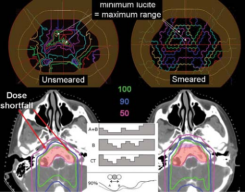 Figure 20.1. The use of range-compensators requires two steps, smearing and tapering, to achieve satisfactory target coverage. Smearing considers each point on the range-compensator and replaces the thickness of that point with the minimum thickness found at other points within a smearing radius of the point under consideration. This has the effect to “throw” the dose deeper into the patient (see bottom-right compared to bottom-left). The middle insert illustrates the example where the CT represents the unsmeared compensator, while B (and similarlly A) is the compensator if a shift were to occur. The composite compensator considers positions A and B. Smearing, originally, was introduced to compensate for geometric uncertainties by considering the “worst”-case penetration range within a region. Tapering considers range-compensator gradients along the aperture edge and applies a smoothing to those gradients to remove scattering artifacts. In general, support for smearing and tapering is poor within existing treatment planning systems and requires considerable knowledge on the treatment planner to achieve a satisfactory result. |
The depth of the Bragg peak is a function of the initial proton beam energy and there is a direct correspondence between energy E (in MeV) and penetration depth or range R (in g/cm2). The terms “energy” and “range” are interchangeable although the range is more effective in clinical communication. A consequence of the energy–range relationship is that the energy loss can be equated to material thickness. Thus, inserting a material of certain thickness in a proton beam results in a proportional energy reduction and a known shift downward of the range. The proton beam intensity, however, does not change: all entering protons exit. This is in contrast to a clinical photon beam where the mean energy is minimally affected while the intensity reduces exponentially as a function of thickness.
The near-straight tracks of the protons produce a beam whose penumbral edge is intrinsically sharp. The individual protons undergo (primarily) many multiple Coulomb scattering events, which result in a Gaussian-shaped broadening of an initially parallel proton beam. The Gaussian spread increases with depth and results in a depth-dependent penumbra (80/20%) (see Fig. 20.2 where the penumbra profile increases per depth).
The proton beam penumbra is intrinsically sharper compared to a single photon beam penumbra at depths below ∼18 cm (in water). This single beam penumbra is relevant when one wishes to achieve the sharpest lateral fall-off of dose between the target and a critical structure. Thus, proton beam treatments in the head and neck achieve a sharper lateral fall-off, for example, in a target around the brainstem compared to a photon (intensity-modulated radiotherapy [IMRT]) beam treatment. On the other hand, a prostate or other deep-seated target does not show a penumbral advantage for a proton beam. Of course, other benefits may still favor the proton beam dosimetry.
In practice, however, it is the composite penumbra of multiple fields that is of relevance as it determines not only the sharpest achievable penumbra but also the integral dose “bath” throughout the patient. Photon beams have no localization ability along depth and “pass” through the target. Proton beams, in contrast, deposit no dose beyond the distal edge of the Bragg peak. This simple difference means that a composite of multiple proton beams will have approximately half the integral dose of a similarly arranged set of photon beams (see Fig. 20.3).
A single proton field, as the composite of multiple individual dose-weighted Bragg peaks, can deliver an arbitrary dose distribution to a target volume. Scattered proton fields, in clinical practice, are shaped to deliver homogeneous dose to all or part of the target volume. In the case of partial target coverage, a second field is used to fill-in or “patch” (see below) the remainder. Thus, a single proton
field can achieve the desired dose description. Such a single proton field can achieve superior dose shaping by virtue of the lateral penumbra and the distal fall-off that spares distal tissues. A single scattered proton field cannot control the entrance dose given the fixed modulation width of a spread-out Bragg peak (SOBP). An example of such a field is shown in Figure 20.3 in comparison to an IMRT treatment.
field can achieve the desired dose description. Such a single proton field can achieve superior dose shaping by virtue of the lateral penumbra and the distal fall-off that spares distal tissues. A single scattered proton field cannot control the entrance dose given the fixed modulation width of a spread-out Bragg peak (SOBP). An example of such a field is shown in Figure 20.3 in comparison to an IMRT treatment.
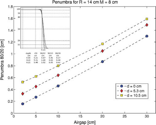 Figure 20.2. The effect of increasing the airgap in a scattered field results in an increase in penumbra because the projection of the effective source size, on the order of 7 cm in scattered proton fields, in the patient increases. The penumbra also increases, but much less so, as a consequence of the scatter in patient as a function of depth (depths of 0, 5.3 and 10.5 cm are shown for a field of 14-cm range and 8-cm modulation). The initial penumbra at a depth of 0 equals the projected source size only as the proton beam has not yet scattered in the patient. The insert (top left) shows the penumbra for this field as a function of depth for an airgap of 5 cm. |
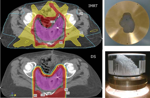 Figure 20.3. Treatment plans, intensity-modulated radiotherapy (IMRT) and scattered fields (DS), for endometrial nodal disease are compared. The IMRT plan uses seven fields and has an unavoidable dose bath (yellow between 50% and 80% isodose lines). The DS plan, in contrast, achieves superior coverage with a single posterior aperture and range-compensator field (examples of these devices, not those used for this treatment, are shown on the right). The aperture, as for a photon beam, achieves lateral beam’s-eye-view conformance. The range-compensator shifts the proton penetration range in proportion to the local thickness to conform the dose to the distal surface of the target volume. Note that for a scattered field, the entrance dose cannot be controlled and results for this case in near, full skin dose. |
The distal fall-off of the Bragg peak has the sharpest dose gradient (about half of the lateral penumbra) and
should offer the best opportunity to achieve a dose differential between target and healthy tissues. In practice, however, the range in patient has an uncertainty estimated on the order of 3.5%. This uncertainty arises from the uncertainty in (relative) stopping power in the patient as derived in practice from CT. CT data measures, per voxel, the electron density in Hounsfield units. For proton radiotherapy treatment planning, the Hounsfield unit in each voxel is converted to stopping power using a tissue-dependent conversion curve (Fig. 20.4). This conversion is empirical and global, and ignorant of patient-specific variations. Proton radiotherapy planning assumes the worst-case scenarios concerning the possible position of the distal edge of the Bragg peak. In practice the distal edge is extended beyond the target volume by 3.5% of the distal range. The modulation, that is, the difference between distal and proximal (90–98%, in our practice), is extended by 7%. Most significantly, it means that the distal edge cannot be used to achieve a dose gradient between the target and a critical structure—doing so could imply a direct overshoot into the critical structure!
should offer the best opportunity to achieve a dose differential between target and healthy tissues. In practice, however, the range in patient has an uncertainty estimated on the order of 3.5%. This uncertainty arises from the uncertainty in (relative) stopping power in the patient as derived in practice from CT. CT data measures, per voxel, the electron density in Hounsfield units. For proton radiotherapy treatment planning, the Hounsfield unit in each voxel is converted to stopping power using a tissue-dependent conversion curve (Fig. 20.4). This conversion is empirical and global, and ignorant of patient-specific variations. Proton radiotherapy planning assumes the worst-case scenarios concerning the possible position of the distal edge of the Bragg peak. In practice the distal edge is extended beyond the target volume by 3.5% of the distal range. The modulation, that is, the difference between distal and proximal (90–98%, in our practice), is extended by 7%. Most significantly, it means that the distal edge cannot be used to achieve a dose gradient between the target and a critical structure—doing so could imply a direct overshoot into the critical structure!
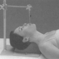
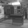
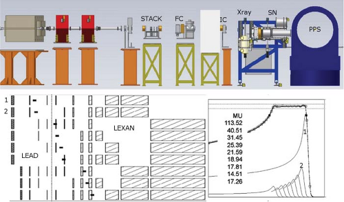 Figure 20.4. The radiosurgery beamline uses a single-scattered proton beam. A stack of lead and lexan absorbers shift and scatter the proton beam (of R = 20.7 cm) to the desired energy and fixed scattering angle. The reference ionization chamber (IC) counts the appropriate number of MU to create spread-out Bragg peaks (SOBPs) of the desired modulation. The patient is positioned on the patient positioner (PPS) at 450 cm from isocenter (the dot in the lamination pattern on left bottom). The position is verified with x-ray and the snout (SN) allows imaging of the full cranial anatomy and with the aperture. The beam energy is verified by a multi-layered Faraday cup (FC). A thick neutron absorber (white) between the FC and IC reduces the neutron dose well below the required levels at the patient. |
Proton dose distributions are biologically equivalent to photon dose distributions except for a constant relative–biological effect (RBE) factor of 1.1. That is, a photon dose of 54 Gy (Co60 equivalent) equals a physical—as measured in an ionization chamber (IC), proton dose of 54/1.1, or 49.1 Gy. Proton dose distributions are, therefore, stated as 54 Gy (RBE) (4) to indicate that the physical dose has been corrected by the RBE factor and can be compared directly to an equivalent photon dose distribution of 54 Gy. Dose effect knowledge from photon radiotherapy can thus be transferred to proton radiotherapy. This is a major advantage in the clinical application of proton radiotherapy. In contrast, the RBE of heavier charged particles, that is, for Lithium and beyond, introduces significant complexities and unknowns in dose reporting.
Generation of Clinical Proton Fields
The proton pristine Bragg peak is too narrow, on the order of 6 mm, to be clinically useful. Thus, many Bragg peaks must be added and distributed through the target volume to achieve a clinical dose distribution.
Accelerators
The generation of a clinical proton beam requires an accelerator to achieve a desirable clinical energy range of up to about 250 MeV. The latter corresponds to about 38 cm in water and is considered good maximum choice given the deepest seated targets. The lowest minimum range is about 3 to 4 cm (60 MeV) and is needed for orbital and other shallow targets.
Current accelerating technologies are cyclotrons and synchrotrons. A cyclotron accelerates a proton beam when
it crosses repeatedly over a gap over which a strong cyclical (of a period equal to the proton traversal time between gap crossings) electrical field is applied. The proton beam is in a constant magnetic field B = BT and the accelerating proton beam assumes an ever-increasing radial orbit R, that is, R = R(E). At the highest design energy, that is, at the maximum radius T = R(EMAX) of the cyclotron cavity, the proton beam is extracted from the cyclotron. Thus, a cyclotron produces a single energy beam EMAX and the proton beam must pass through a carbon or beryllium (i.e., a low scatter material) variable thickness degrader to achieve the desired clinical energy. A synchrotron accelerates the proton beam by passing it through an accelerating cavity and keeps the beam in a constant-radius orbit T by synchronizing (and increasing) the magnetic field with the proton energy, that is, B = B(E) such that the proton bending radius equals T. A synchrotron can produce any energy E, proportional to the number of passes through the cavity and limited by the maximum magnetic field B, without the need for post-extraction degradation.
it crosses repeatedly over a gap over which a strong cyclical (of a period equal to the proton traversal time between gap crossings) electrical field is applied. The proton beam is in a constant magnetic field B = BT and the accelerating proton beam assumes an ever-increasing radial orbit R, that is, R = R(E). At the highest design energy, that is, at the maximum radius T = R(EMAX) of the cyclotron cavity, the proton beam is extracted from the cyclotron. Thus, a cyclotron produces a single energy beam EMAX and the proton beam must pass through a carbon or beryllium (i.e., a low scatter material) variable thickness degrader to achieve the desired clinical energy. A synchrotron accelerates the proton beam by passing it through an accelerating cavity and keeps the beam in a constant-radius orbit T by synchronizing (and increasing) the magnetic field with the proton energy, that is, B = B(E) such that the proton bending radius equals T. A synchrotron can produce any energy E, proportional to the number of passes through the cavity and limited by the maximum magnetic field B, without the need for post-extraction degradation.
The primary difference between a synchrotron and cyclotron is the need for energy degradation of the latter. The degrading material, however, scatters the beam, which results in a large emittance, that is the position and momentum phase space, for a cyclotron. This, in turn, affects the beam transport design and the ability to achieve a narrow beam at the patient. The choice of cyclotron was preferred due to their simpler operation and higher beam current. The latter is to compensate for proton loss in scattered fields where a large portion of protons (between 50% to 90%) is lost to scatter and field collimation within the scattered field radius. The emerging preference for scanned beam technology, however, places different requirements on the beam parameters compared to scattered beams and the choice between synchrotron and cyclotron may shift in favor of the synchrotron.
The generated beam is transported to the treatment delivery device using a magnetic beamline. A distributed beamline allows a single accelerating device to supply multiple treatment rooms which reduces the overall facility cost.
Scattered Proton Fields
An initially narrow proton beam of a given energy is shifted to lower energies and spread in depth by different thickness absorbers, broadened and flattened laterally by carefully designed scatterers, and “stacked” with appropriate weights by synchronizing absorber insertion with monitor units (MU) or another integrated beam-current measure (see Fig. 10.2). Such composite and scattered proton fields are labeled SOBP fields and, in general, produce homogeneous dose per field over a desired modulation width up to a maximum range.
Related posts:

Stay updated, free articles. Join our Telegram channel

Full access? Get Clinical Tree


