Patient and Organ Movement

James M. Balter

Introduction

The driving tenet of conformal radiotherapy is the precise delivery of focal radiation doses to the target, so that an effective dose can be delivered while limiting concomitant normal tissue irradiation and related toxicity risk. Technical advancements, such as three-dimensional (3D) treatment planning and intensity-modulated radiation therapy (IMRT), have provided significant gains in specifying means to provide such dose distributions. Accurate delivery, so that intended and actual doses agree, is a more complicated matter.

The problems of patient positioning and motion have been studied extensively. Although there are currently areas that need further exploration, it is possible to consider the magnitude of various uncertainties in dose delivery due to patient position variation and organ movement, and to discuss rational strategies for dealing with these uncertainties in the context of precision radiotherapy.

Description of the Problem of Geometric Variation

The International Congress on Radiological Units (ICRU) has addressed the relative problem of geometric variations. In reports 50 and 62, concepts are evolved to attempt to standardize means of reporting doses. Some of the concepts presented in these reports have served as the basis for numerous investigations over the past few years, and have been adopted as standards for clinical trials. A brief discussion of the key concepts as they apply to geometric variation follows.

The key structures that are delineated are the gross tumor volume (GTV) and organs at risk (OARs). The GTV is generally defined as the “visible” target, that is, that can be delineated from imaging or related information. The OARs are tissue structures that are dose limiting due to risk of radiation-induced toxicity.

The next volume of interest is the clinical target volume (CTV). This target volume ideally expands about the GTV to include a reasonable expectation of the true target extent on a (static) patient model. The basis for CTV expansions includes intraobserver and interobserver variations in tumor delineation, as well as a reasonable expectation of the extent of disease below the sensitive range of the imaging modality.

Geometric uncertainty influences both the target volume and the OARs. To ensure adequate geometric coverage of the target, the CTV is expanded. Internal organ movement is encompassed by an internal margin (IM) about the CTV to make the internal target volume (ITV), and setup error influences a setup margin (SM) about the ITV to yield the planning target volume (PTV).

When the patient is imaged to define the CTV and critical structures, the position is sampled. In general, this sample occurs once, specifically during the computed tomography (CT) scan for treatment planning. To obtain this sample, the patient is immobilized and positioned with typical reference marks placed on the skin and/or immobilization device at the principal axes of the CT scanner for verification of position and orientation. The sample of the patient serves as the model for treatment planning, and all subsequent targeting and density modeling are based on the information obtained during this session.

Suppose the patient has the same treatment planning scan repeated several times over the course of a typical fractionated treatment regimen (4–8 weeks). With no prior reference to positioning (i.e., no attempts to match the reference marker positions from one CT scan to the next), each CT scan will yield a patient model that differs in both position and configuration. These variations may be slight (indicating good reproducibility of patient position) or severe. Let us now suppose that attempts are made to reproduce the position of the patient so that the external reference marks line up relative to the CT scan lasers. This process, which in effect simulates multiple positioning by the “3-point setup” method to external references, will still yield a variety of patient positions and configurations in the CT scans obtained. The variation in these scans determines the extent to which external references properly configure and position the patient.

The magnitude of position variation has been studied by several hospitals over the past two decades. Table 4.1 (1,2,3,4,5,6,7) highlights some of these measurements, and indicates a reasonable range of expected variations. Note, however, that these reported values are unique to specific hospitals, immobilization equipment, and procedures. They are also influenced to a lesser extent by the means of
measuring position variation. It is critical that a department determines its own position variation distributions, both as a baseline for treatment planning and as a means of improving positioning in an efficient manner.

Table 4.1 Example Measured Setup Variations

Investigator	Body site	Nature of measured setup variation
Hong et al.	Head/neck	Mean error 6.7 mm, σ 3.63 mm
Michalski et al.	Various	6% of monitored fractions with errors >10 mm
Meijer et al.	Bladder	3 mm (1 σ)
Marsh et al.	Head/neck	Range of up to 4.5 mm (5 w into treatment)
Pisani et al.	Various	Mean error of 6.6 ± 2.4 mm
Weber et al.	Prostate	1.9–2.2 mm (systematic), 3.6 mm (random)
Van de Steene et al.	Thorax	Random σ 4.5-mm longitudinal and 5.7-mm transverse

Multiple samples of patient position (translation only) will form a scatter distribution. If we accept the position from the initial (treatment planning) CT scan as the “true” patient position, then a reasonable method of describing this distribution of subsequent positioning is by the translation necessary to make the patient position match that of the treatment planning CT scan. Conventionally, the average coordinate of this distribution is considered as the “systematic” error, in that it is the effective offset that persists throughout the samples (multiple CT scans in the above example, or multiple patient positions over a course of treatment). The spread of sampled positions about this average coordinate represents the random setup variation. It is important to note that the average coordinate may never be sampled.

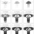
Figure 4.1 shows a scatter distribution of patient position over multiple samples (about two axes), relative to the treatment planning CT scan representation of a patient. Note that the treatment planning CT scan does not reflect the average position or configuration of the patient. At best, it is just one of the random samples of position. At worst, due to patient discomfort or unfamiliarity with the immobilization equipment and process, it is a very biased sample of the later position distribution. Nonetheless, the patient at simulation generally reflects the model that subsequent positioning and localization attempt to match.

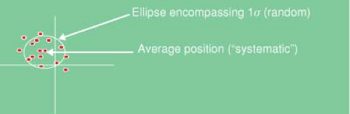Figure 4.1. Scatter distribution of patient position over multiple samples (about two axes), relative to the treatment planning computed tomography representation of a patient.

Let us consider positioning to be described by a Gaussian probability density function. By this assumption, the “average” magnitude of error in any sample is of the order of 0.8 σ, or 80% of the magnitude of the standard deviation of the distribution. Extending this model, it can be shown that the typical magnitude of difference between any two samples of the distribution is approximately 1.1 σ.

Table 4.2 shows some sample random variations measured from patients positioned and evaluated through daily imaging.

There are a number of assumptions that are critical to this simple model. One of the most important is that no time trend exists in patient position. This may not be true in all cases, and time trends in position have been investigated for various body sites.

Minimizing the Impact of Setup Variations on Treatment

Obviously, these setup variations require margins to ensure proper target coverage. The expansion of the CTV to ensure adequate coverage includes a SM to yield the PTV. Reducing the SM yields a smaller volume of tissue
irradiated to high doses, and can potentially reduce the toxicity to normal tissues. As such, significant efforts have been made to minimize the range of variations and their resulting impact on treatment.

Table 4.2 Random Variations in Position Measured from Daily Imaging of Patients for Various Body Sites

Site	Average σ (mm)	Range of σ (mm)
Pelvis	3	1–7
Head and neck	2	1–5
Chest	4	1–12

Positioning Systems

A significant variety of equipment is in use to aid in repeat setup of patients. This equipment attempts to address a dual role: immobilization and localization. These dual roles are not necessarily compatible for any given piece of technology.

Immobilization

Quite simply, the process of immobilization involves limiting or eliminating movement for the time period of imaging or treatment. The primary objective is to limit target movement, although critical normal tissue movement also needs to be considered.

A number of excellent reviews of immobilization equipment have been published recently. As the technology is evolving, however, it is important to consider a number of key aspects in deciding on a technology and strategy for use of an immobilization system.

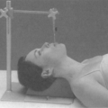
The advantage of a given immobilization method may be compromised by the complexity of use. If an immobilization system has many degrees of freedom, improper configuration of the device may lead to systematic errors in patient position or shape at treatment. Examples of complex systems are multiuse boards for fixation, in which the angles and positions of arm supports, angle of the upper thorax, shape of neck support, and other components are adjustable. These devices are very cost-effective, and can be used effectively, but special care must be taken to properly verify the per patient configuration, including notation of all configuration parameters and documented photographs of proper setup.

Some systems (e.g., alpha cradle and vacuum loc) form directly to the patient’s shape. This can be beneficial in positioning, but it is important to separate comfort from immobilization. Formed immobilization that extends to distal regions from the target has been shown to be beneficial in reproducing position (8).

Localization Technology

A wealth of technology has been applied to localization in radiation therapy. At present, the most prevalent technology includes in-room lasers and electronic portal imaging devices (EPIDS). Improved image quality and ease of use, as well as better software for image review and management have led to EPIDS replacing film as the standard method of setup verification.

Megavoltage radiography is inherently limited by a lack of contrast, and has further been practically limited by the radiation doses involved. Other localization technologies have been introduced to overcome these limitations.

In-room diagnostic radiography is, in fact, a very old concept. Film-based radiographic systems have existed on linear accelerators for over 20 years (9). Room-based digital systems have been used for radiographic (10,11,12,13) and fluoroscopic (14) procedures.

Strategies for Position Correction

Online

Generally, online position correction refers to the processes of measuring and correcting setup error at the start of each treatment fraction. This is the area in which the vast majority of technical developments have focused recently. The process of online correction includes three steps: measurement, decision, and adjustment. A fourth step (verification) may also be used.

Measurement systems include data collection and analysis. Data can be from imaging (e.g., radiographs, CT scan images, ultrasound, and video) or other markers (e.g., electromagnetic and external fiducial). Analysis is the comparison of reference image or position information to that gathered at treatment.

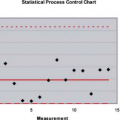
Decision is the process of choosing to act or not on information from measurements. It is valuable to consider that the measurement systems as well as correction technology are not perfect, and therefore the errors in these systems may increase errors in certain circumstances. The use of thresholds for corrections allows a trade-off between the cost (frequency of adjustment) and benefit (actual reduction of errors). Figure 4.2 shows the cost versus threshold for setup adjustment in prostate patients.
Figure 4.3 shows the impact of positioning strategy on margins under assumptions of systematic error versus none.

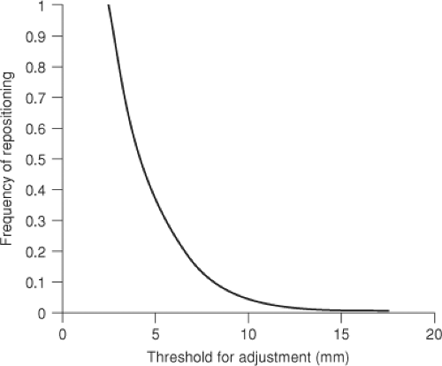Figure 4.2. Cost (frequency of adjustment) versus threshold for online setup adjustment (based on 6-mm σ for pelvic patients).

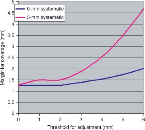Figure 4.3. Benefit (margin) versus threshold for adjustment (4-mm σ setup, 1.5-mm σ measurement uncertainty, and 1.0 mm σ setup correction uncertainty).

Off-line

Studies of the dosimetric impact of setup error (15,16,17,18) demonstrate that systematic error has the largest impact on margin needed to adequately dose a target, and that the geometric expansion to account for random error is generally small (less than one standard deviation). Given this observation, it can be seen that, as long as random errors are not exceedingly large, the most significant patient benefit comes from strategies that rapidly reduce the magnitude of systematic setup variation.

A number of strategies have been used to minimize systematic error. Two common strategies are the shrinking action level (SAL) and no action level (NAL) methods (19,20,21). In the SAL protocol, setup is verified daily for the first few fractions, and adjustments are made with tolerances that reduce in magnitude as the fractions progress. This strategy has shown promising results.

Only gold members can continue reading. Log In or Register to continue