Chapter 5
Modeling Spiking and Secretion in the Magnocellular Vasopressin Neuron
Duncan J. MacGregor and Gareth Leng
Centre for Integrative Physiology, University of Edinburgh, Edinburgh, UK
5.1 Background
5.1.1 Neurons, physiology, and modeling
Magnocellular vasopressin neurons, together with their oxytocin-secreting neighbors, have been important “model systems” in neuroscience because of circumstances that make them exceptionally open to experimental study. The supraoptic nucleus contains only oxytocin and vasopressin neurons, and this greatly facilitates identifying these neurons to make recordings of their electrical activity. Most importantly, however, these neurons all project to the pituitary gland, so their primary output can be measured directly, in their respective plasma oxytocin and vasopressin concentrations. Thus, these systems are a “window on the brain”, they allow us to look directly at the relationship between spiking activity and physiological function.
The first recordings of vasopressin cells announced an enigma that has provoked speculation ever since. In the rat, vasopressin cells display a distinctive phasic firing pattern that is not seen in oxytocin neurons (Figure 5.1). Many types of neurons fire in bursts, but the slow, intrinsic, phasic bursting of vasopressin cells was different from that of other neuronal populations, which mostly exhibit much faster, or network-dependent, bursting. Understanding how vasopressin cells burst, thus, became an important modeling target. Moreover, because of the transparency of their physiological function, combined with diverse opportunities for prediction and testing, it should also be possible, aided by models, to answer why these cells burst.
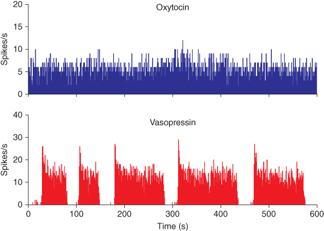
Figure 5.1 Spiking in oxytocin and vasopressin neurons. These traces show 10 min of spiking recorded from typical oxytocin and vasopressin neurons. The activity in the oxytocin neuron is mostly random. The vasopressin neuron shows a “phasic” pattern of long bursts and silences, with a distinctive peak at the start of each burst.
There have thus been many attempts to model these neurons, and both the successes and failures have formed useful steps in learning how to apply modeling to spike and pattern generation. We have developed a computational model which can reproduce the detailed firing behavior of vasopressin cells (MacGregor and Leng, 2012).
5.1.2 History matters
Most modeling papers present the finished product. This is fine if you want to know what it contributes to the physiology, or to use it as a tool, but to learn how to model, or to assess how good a model is, it helps to understand exactly how the model ended up in its final form. The final model would have been preceded by many earlier versions, even whole previous models which never made it to publication. These hidden parts can be useful to other modelers, and can also help give more confidence in the final model to the physiologists. Here, we present this story for the vasopressin neuron.
5.1.3 Detection and recording
The rat hypothalamus contains about 9000 magnocellular vasopressin neurons, mostly within the supraoptic and the paraventricular nuclei. The supraoptic nucleus contains only magnocellular neurons, about 70% of which make vasopressin and 30% oxytocin. Because all magnocellular neurons project to the posterior pituitary gland, and because only magnocellular neurons project there, it is possible to identify these neurons antidromically: if a stimulating electrode is placed on the neural stalk through which all axons en route to the pituitary pass, then stimuli will trigger spikes in those axons; these spikes are propagated antidromically to invade the cell bodies, with a latency that reflects the axonal length and the propagation speed.
Oxytocin cells and vasopressin cells can be distinguished from each other not only by their responses to various stimuli, but also by their spontaneous firing patterns (Figure 5.1). Most importantly, many supraoptic neurons fire in a phasic pattern, and these are almost always vasopressin cells. Phasic bursts typically begin with a rapid acceleration to a peak firing rate as high as 30 spikes/s; this peak only lasts a few seconds, subsiding to a plateau firing rate of at least 4 spikes/s and up to 10 spikes/s. The bursts usually last for 10–60 s, end abruptly, and are followed by (typically) 10–30 s of silence, punctuated by just the occasional spike. In any one cell, the pattern tends to be quite consistent, though with more variability in burst duration than in silence duration.
During lactation, oxytocin neurons also fire in bursts, but these are very unlike the bursts of vasopressin cells. In response to suckling, at intervals of several minutes, oxytocin cells synchronize to produce a short (1–3 s) and intense (50–100 spikes/s) burst of spikes that leads to a large pulse of oxytocin secretion, driving milk ejection. In contrast, the phasic firing in vasopressin neurons is asynchronous; even adjacent cells show no correlation in their spiking activity. Therefore, the population output is not phasic, and so if there is any purpose to phasic firing, it is not for generating patterning in the final output.
5.1.4 In vivo versus in vitro
Our focus is on modeling the activity of vasopressin neurons in vivo (in anaesthetized rats), but our model must be reconciled with data obtained both in vivo and in vitro. However, there are differences between the behavior of vasopressin cells in vivo and in vitro (and differences between in vitro hypothalamic slice preparations, hypothalamic explants, isolated cell preparations, and organotypic cultures). Many of these differences relate to the sparseness of synaptic input in vitro. The few intracellular recordings that have been made in vivo confirm that supraoptic neurons in vivo receive intense synaptic input, whereas vasopressin neurons in vitro typically receive very little. In slice preparations, magnocellular neurons have truncated dendrites, few of their sources of input remain within the slice, those that are may not still be connected to the vasopressin neurons, and those that do remain are themselves deafferented. The neurons still generate spikes in response to direct depolarization, but show little spontaneous spiking unless the bathing medium is adjusted by, for instance, an increase in K+ concentration or by the addition of glutamate.
This is a general issue with in vitro recordings; an intact neuron in the brain may receive 10000 synaptic inputs, and if most come from active neurons, then they receive a massive barrage of excitatory and inhibitory synaptic potentials (EPSPs and IPSPs). Because most classical neurotransmitters open ligand-gated ion channels, the overall conductance state of the neuron at rest is different in vivo and in vitro; a high rate of input results in extensive opening of ion channels, reducing the cell’s input resistance, with consequences for many membrane properties. The effect of the voltage-gated opening of ion channels depends on the cell’s input resistance; if this is high, then a given change in conductance will produce a larger change in membrane voltage. Accordingly, activity-dependent mechanisms are exaggerated in in vitro preparations; these preparations give good access to the components of the spiking mechanism, but properties such as the magnitude and time course of voltage-dependent conductances may be altered.
Over and above this, the membrane noise that synaptic input provides can change how neurons process information. We often assume that noise is undesirable, but in complex nonlinear systems “stochastic resonance” can occur. Stochastic resonance is when an increase in levels of unpredictable fluctuations improves the quality of signal transmission or detection performance, rather than degrading it, raising the possibility that the brain has evolved to utilize random noise as part of the “neural code.” Stochastic resonance is an essential part of osmoresponsiveness in vasopressin neurons. Vasopressin neurons possess stretch-sensitive ion channels that support depolarization in response to the cell shrinkage that accompanies a rise in extracellular osmolarity. In the physiological range of osmotic stimuli, this depolarization is too small to result in spike activity in vasopressin cells that are isolated from a synaptic input. However, the presence of fluctuations in membrane potential changes this – even a small depolarization will increase the probability that fluctuations will exceed spike threshold, allowing small sustained depolarizations to translate into increased spiking activity.
Thus, synaptic “noise” is not merely something that adds imprecision to the behavior of a neuron; it can alter how the neuron processes information. To model vasopressin cells as they operate physiologically, we must include a realistic simulation of synaptic noise. We can incorporate intrinsic mechanisms as established by in vitro experiments, but must be aware that the magnitude and dynamics of conductance changes will be different in vivo from those observed in vitro.
5.1.5 Outputs
Vasopressin cells project to the posterior pituitary gland, where spike activity triggers exocytosis of hormone-containing vesicles. The peptide secreted from the nerve terminals of the 9000 vasopressin cells forms a relatively smooth summed signal, which passes into the bloodstream and on to targets across the body. This is the important output, the population signal, and to understand the function of the phasic firing pattern, we must recognize that the pattern of secretion from any single cell is lost in the output of a large and asynchronous population.
In many neuronal network models, it is assumed that the output of neurons is synonymous with their spike activity. But the biologically relevant output of any neuron is not its spike activity, but the chemicals that it secretes. This secretion is regulated by spike activity, but the relationship is not linear, is state dependent, and often is subject to retrograde modulation by factors secreted from the post-synaptic target. Thus, the presumption that spike activity is an adequate representation of the information transmitted from a neuron is always unsafe. However, for vasopressin cells, we know the properties of stimulus–secretion coupling, and so we can relate our understanding of spiking behavior to the real output of these neurons.
5.1.6 Asynchronous bistability
Vasopressin cells in vivo are not spontaneously active; without synaptic input, they remain silent. With low rates of synaptic input, they exhibit very slow ( 1 Hz) or irregular spiking. However, given enough synaptic input, they fire phasically. This is not because the input comes in a phasic pattern. Phasic firing involves a combination of activity-dependent excitation and a delayed activity-dependent inhibition. Activity-dependent excitation of bursts can be demonstrated by perturbing a vasopressin cell during its silent period with a stimulus strong enough to trigger just a few spikes. Such stimuli will trigger the onset of a burst depending (a) on the intensity and (b) on the time that has elapsed since the end of the previous burst: it becomes progressively easier to trigger a burst with increasing time. Activity-dependent inhibition can be observed similarly, by delivering stimuli during a burst. Stimuli will stop a burst depending (a) on the intensity and (b) on the time that has elapsed since the beginning of the burst: it becomes progressively easier to stop a burst with increasing time. Thus, the same stimulus can stop or start bursts depending on exactly when in the burst cycle it is delivered. This identifies the vasopressin cell as a bistable oscillator – it has two relatively stable states, activity and silence, and even small perturbations can “flip” the cell from either state into the other.
Knowing that vasopressin cells fire asynchronously, we can see that a brief stimulus may activate some cells, inhibit others, and have no effect on many – and which cells it activates and which it inhibits depend purely on the state of the different cells at the time of application. Phasic activity in vasopressin cells, therefore, does not depend critically on the patterning of their inputs and must be generated by an intrinsic mechanism. However, excitatory inputs are essential for any spiking in vasopressin cells in vivo, and these inputs can be modulated by several retrograde signals that are released from the dendrites of vasopressin cells. So in some circumstances, the input to vasopressin cells is correlated with the phasic activity, but it is the phasic activity that determines the input pattern, not the input pattern that determines the phasic pattern.
5.2 Modeling
5.2.1 Inputs, and a good place to start a model
The inputs to vasopressin cells are diverse, reflecting the multiple functions of vasopressin. Some inputs come from osmoresponsive neurons of the forebrain, including from two “circumventricular organs” – the subfornical organ (SFO) and the organum vasculosum of the lamina terminalis (OVLT). These inputs involve both excitatory inputs mediated by the neurotransmitter glutamate and inhibitory inputs mediated by gamma-aminobutyric acid (GABA).
Synaptic input consists of many small events. We expect a typical neuron to receive inputs from many different neurons, via as many as perhaps 10000 synapses. Assuming that these inputs are independent on a short timescale (tens of milliseconds), the timing of each synaptic event is essentially random. This gives us a simple way to simulate the spontaneous inputs for a model neuron, by using a random number generator to generate inputs, using a defined mean rate. Each input event generates a postsynaptic potential (PSP) which rises rapidly over 1–2 ms, to a magnitude of  1–5 mV and then decays more slowly, over 10–20 ms. These PSPs can be either excitatory (depolarizing) EPSPs or inhibitory (hyperpolarizing) IPSPs. Because the rise is rapid, we can simplify the PSP to an instantaneous step and model the decline using a single exponential decay. PSP magnitude varies between synapses and events, and also depends on the difference between the membrane potential and the reversal potential for the ion that carries the PSP (usually mainly Na+ for EPSPs and Cl− for IPSPs). Just after a spike, IPSPs are smaller because the vasopressin cell is hyperpolarized, but because of this hyperpolarization, the vasopressin cell is not spiking then, so the difference in IPSP size has no consequences for spike activity. Otherwise, changes in PSP magnitude are small, and if we simplify by using a fixed magnitude for PSPs, we do not affect anything noticeably. It is always worth checking conclusions using a detailed model with variable PSP magnitudes and half-lives, and with realistic reversal potentials, but in our models of vasopressin cells, qualitative behavior is robust to such changes. Hence, in our working model, synaptic input is defined by just three parameters for EPSPs and three for IPSPs: event rate, magnitude, and decay rate. If we make these the same for EPSPs and IPSPs, we can study the neuron under conditions where the input is, on average, an exact balance between inhibition and excitation – the state at which we expect neurons generally to be, in resting conditions in vivo, given that we know that inhibitory synapses and excitatory synapses are approximately equally abundant on magnocellular neurons.
5.2.2 Membrane potential
Hodgkin–Huxley-type models model a cell’s membrane potential in detail, using representations of the dynamics driving individual ionic conductances. In contrast, in the integrate-and-fire (or spike-response) model, we only model influences on the neuron’s ability to fire a spike (its “excitability”). The first of these “influences” are the PSPs. Each of these perturbs the membrane potential, which starts at a fixed resting value (the resting potential). If the membrane potential reaches a spike threshold, we record a spike. We do not model the spike’s rapid changes in the membrane potential, only record its time of occurrence, but we do model the slower changes in the membrane potential which follow.
5.2.3 Post-spike potentials
The other “influences” consist of potentials generated by the cell after a spike. Vasopressin neurons express several types of voltage-gated Ca2+ channels, and every spike is accompanied by Ca2+ entry. Accordingly, repetitive spiking results in a large increase in intracellular (cytosolic) Ca2+ concentration ([Ca2+]i). This is cleared quite slowly, and it functions as a short-term memory of spike activation, influencing membrane properties via Ca2+-sensitive channels. There are several types of Ca2+-sensitive channels, and their time course and magnitude of activation differ, depending on channel properties, spatial distribution, proximity to the Ca2+ entry channels, and variable Ca2+ dynamics within the cell.
In vasopressin neurons, we can recognize three phases of post-spike-altered excitability that we can relate to these channels (Figure 5.2). Immediately after, and for about 30–40 ms, is a period of relative inexcitability, which reflects a hyperpolarizing afterpotential (HAP), mediated by a voltage- and Ca2+-dependent K+ current. This is succeeded by relative hyperexcitability, which is the result of a voltage- and Ca2+-dependent depolarizing afterpotential (DAP), which has both a fast and a slow components. Finally, trains of spikes activate a long-lasting reduction in excitability, identified with a Ca2+-dependent afterhyperpolarization (AHP) that has both an apamin-sensitive, medium duration component and a slower, apamin-insensitive component.
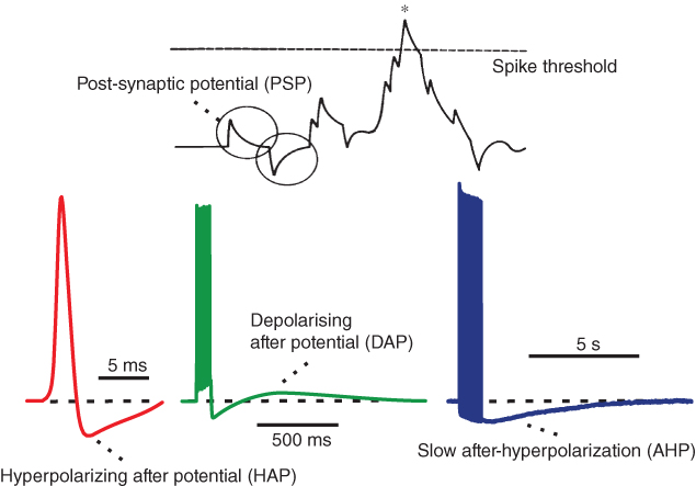
Figure 5.2 Integrate-and-fire and afterpotentials. Model simulated excitatory and inhibitory PSPs summate and trigger a spike when the sum (the membrane potential) crosses the spike threshold. Following the spike, the HAP, DAP, and AHP are simulated by decaying exponentials with varied magnitude and half-life.
We can either model these post-spike potentials as conductances in a Hodgkin–Huxley-type model, or model the changes in excitability as a function of spike activity in a spike-response model. Which approach we choose depends on exactly what data we are using to fit the model and what behaviors we are trying to explain. Here, we are interested in understanding the genesis of spike-activity patterns and their role in information processing, and our data come from extracellular recordings of spike activity in vivo. Accordingly, we are not primarily interested in the shape of spikes and are less interested in how the HAP, DAP, and AHP are formed than in their influence on spike patterning. We want a model that is inspired by the biophysical understanding from mechanistic in vitro studies, but quantitative data derived from in vitro studies cannot easily be used in a model of in vivo behavior because of the caveats referred to above.
A spike-response model uses deterministic functions that describe the effects of spike activity, rather than the underlying mechanisms, and hence can be computationally concise. Such a model aims only to match spike-timing data. For vasopressin neurons, the HAP, DAP, and AHP are the result of a superposition of spike-triggered conductance changes that have different dynamics. In a spike-response model, we model these as exponentially decaying changes in the membrane potential, and, for any given vasopressin cell, we can choose parameters for these that generate a model that is effectively indistinguishable from the recorded cell by statistical measures of spike activity.
5.2.4 Spike analysis
We fit the model by applying the same analysis techniques that we use to examine the experimental data. Our analysis of experimental data begins with the series of spike times from cells recorded in vivo. It is possible to record spike activity from a single vasopressin cell for several hours, and, because extracellular recording does not involve damaging the cells membrane integrity, activity patterns are very stable. For a cell firing at a mean rate of 5 spikes/s (about average for vasopressin cells recorded in vivo), 1 h of recording yields a time series of about 18000 spike events.
From the spike times, we calculate the interspike intervals (ISIs) and generate an ISI histogram, showing the ISI distribution (Figure 5.3). If a cell has an equal chance of firing a spike at any time, that is, if spikes occur purely randomly, then the ISIs will follow a Poisson distribution – the number of ISIs of a given length declines exponentially with increasing length. However, this cannot be exactly true for any neuron: every neuron has an absolute refractory period when it cannot fire again after a spike, and there can be no ISIs less than about 2 ms. After the absolute refractory period, neurons have a relative refractory period, but the duration of this varies considerably between neuron types. A refractory period manifests as an obvious gap at the front of the ISI distribution (Figure 5.4), but other effects on the ISIs tend to be lost in the curved Poisson tail of the distribution, and are better detected using the hazard function. The hazard function is generated by transforming the ISI distribution into a plot of the probability of a spike occurring as a function of the time elapsed since the last spike (Sabatier et al., 2004). The curved Poisson tail becomes a flat plateau, and any deviation from a constant hazard value indicates an effect of the spike on neuronal excitability (Figure 5.4).
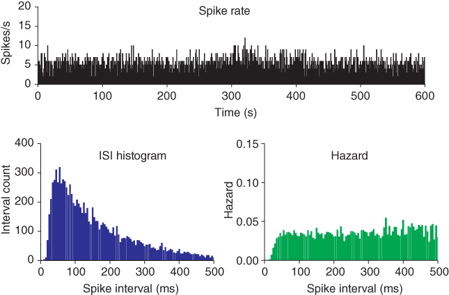
Figure 5.3 Inter-spike interval (ISI) histogram and hazard oxytocin cell example. These show short-term patterning in the spike activity. The hazard becomes less reliable at longer intervals, but a good hazard function can usually be generated for up to  500 ms, subject to the firing rate and number of spikes in a recording.
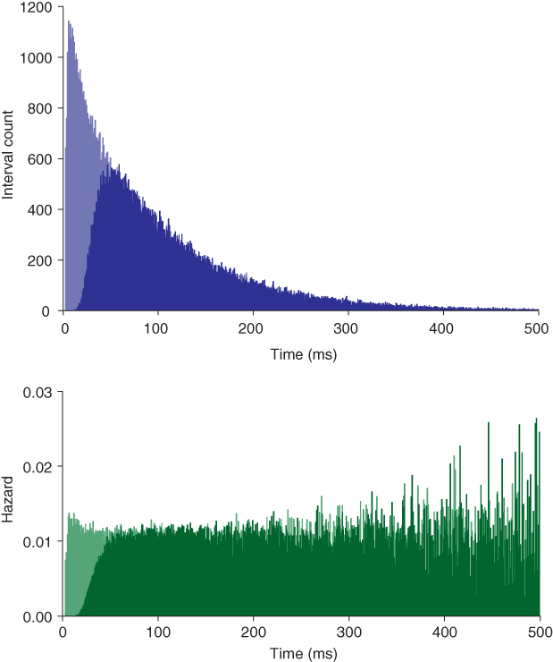
Figure 5.4 Model fitted to oxytocin cell. The dark shaded histogram and hazard show the basic model with an HAP fitted to the oxytocin cell of Figure 5.3. The light shade shows the effect of removing the HAP (hyper-polarizing afterpotential). Spiking is then only limited by the absolute refractory period (2 ms). The small peak early in the hazard shows a small increase in post-spike excitability due to the persistence of EPSPs (excitatory post-synaptic potentials).
5.2.5 A simple model
The HAP, in both oxytocin and vasopressin cells, is a spike-triggered hyperpolarization which decays over about 30–40 ms (Figure 5.2). The first published spiking model studying these cells (Leng et al., 2001) focussed initially on the simpler spike patterning in oxytocin neurons, represented synaptic input as randomly generated PSPs and the HAP as a fixed, step change, that occurs instantaneously with a spike, which subsequently decays exponentially (Figure 5.5), and defined by just two parameters, step magnitude and half-life ( and
and  ). This simple model matched the ISI distributions and hazard functions of oxytocin cells indistinguishably, showing that a simple HAP is sufficient to explain the observed refractoriness in oxytocin cells.
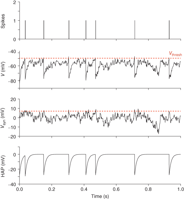
Figure 5.5 Traces of the simple oxytocin cell model.  shows the summed random EPSPs and IPSPs. These are summed with the fixed
  to generate the membrane potential
  . When this crosses
  the model records a spike and increments the HAP, which is also summed with
  , generating a post-spike refractory period.
5.2.6 Slower effects: the AHP
Slower effects that last beyond a single ISI and summate over a train of spikes may not be apparent in the ISI distribution, and are still difficult to distinguish in the hazard. The AHP is much smaller than the HAP, but has a much longer half-life ( 500 ms), and its effects can be identified by plotting ISI duration against the mean preceding ISI duration (MacGregor et al., 2009). If ISIs are independent of previous activity, then this will show no correlation (Figure 5.6); but in oxytocin cells, there is a weak inverse correlation, indicating that short ISIs are more likely to be followed by longer ISIs and vice versa. This effect accumulates, so a train of short ISIs is increasingly likely to be followed by a long ISI. The HAP, in comparison, is usually much shorter than a single ISI, and so cannot summate during a train of spikes. Thus, although both the HAP and AHP are hyperpolarizing influences, their different magnitudes and time courses give them different roles.
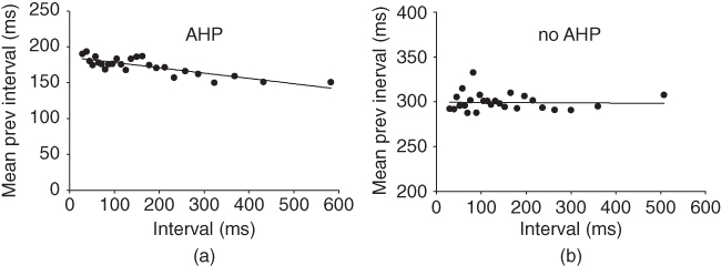
Figure 5.6 Detecting the AHP’s influence using spike train analysis. Adding an AHP to the simple model and applying spike train analysis to the spike times shows a negative correlation (a), matching the same analysis applied to a recorded cell. With no AHP the model can still match the ISI histogram and hazard, but not the negative correlation (b).
The role of the AHP in this “spike ordering” effect was tested with the model (MacGregor et al., 2009), using the same decaying exponential form as the HAP. The model fitted to cell data with just an HAP matches the ISI histogram and hazard, but does not show the spike-ordering effect. Adding an AHP to the model had a greater negative effect on the spike rate than expected, requiring a higher rate of synaptic input to refit the cell data, but otherwise had little effect on the fit to the ISI histogram and hazard function. It did, however, reproduce the spike-ordering effect observed in the oxytocin cell data, suggesting that it is indeed the AHP which is responsible. Functionally, the AHP in oxytocin cells acts to stabilize a cell’s firing rate in that randomly occurring flurries of spikes are immediately compensated for by a counterbalancing depression of activity.
5.3 Bursting in a spiking model
5.3.1 Detecting bursting
The same type of model can also be fitted to the spike rate, ISI histogram and hazard of vasopressin neurons. However, it only matches the short timescale patterning, not the bursting. Approaching this problem first of all requires quantitative detection. Analysis techniques such as the hazard function and spike train analysis can be used to detect short timescale spike patterning which cannot be visually observed. Longer timescale patterning, such as phasic firing, can be crudely detected visually, by counting the number of spikes per second and plotting spike rate against time (Figure 5.1). However, for quantitative detection and analysis of phasic bursts, we use an algorithm which scans through the whole sequence of spike intervals, defining a burst by two criteria:
- a burst contains at least
 spikes
- no ISI within the burst is greater than
 ms.
ms.
For vasopressin cells, we use  and
and  , but by varying
  and
and  , this method can be adapted to detect bursting on multiple timescales, even when bursting exists at multiple scales within a single recording, such as in mitral olfactory neurons. A useful visual analysis technique is to use the time points of the detected bursts to color the spike rate plot, so that the algorithm can be checked against visual identification (Figure 5.7).
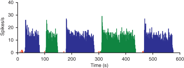
Figure 5.7 Using coloring to visualize burst detection. If you are developing your own software then simple coloring is a very useful tool for visualizing bursts and adjusting the detection parameters. The alternating green and blue make it easier to see where detected bursts begin and end.
5.3.2 How does bursting work?
The key mechanism underlying phasic bursting is the DAP, which is slow enough to summate across ISIs, and by causing faster spiking, acts as a positive feedback. The presence of a DAP in vasopressin cells (but not generally in oxytocin cells) can be recognized from the hazard function, where the DAP is reflected by a peak following the HAP. The hazard function shows the sequence of post-spike effects: first the HAP, then the DAP, eventually followed by the AHP, which if large enough can be observed in the hazard as a slow, positive gradient (Figure 5.8).
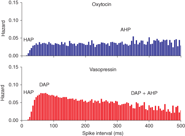
Figure 5.8 Oxytocin versus vasopressin hazard – post-spike influence of the DAP. The DAP generates a peak in the hazard, observed in vasopressin, but not oxytocin neurons. The peak indicates a period of increased post-spike excitability following the decay of the HAP. At longer intervals the influence of the DAP in the vasopressin hazard competes with the AHP. In the oxytocin hazard, the AHP manifests as a very gradual positive slope following the HAP.
The earliest hypothesis for the burst mechanism was that the DAP generates a “plateau potential” which maintains the burst. The positive-feedback effect would initially generate a rapid increase in the spike rate, which would then reach a limit at a level sufficient to allow enough spiking to maintain the “plateau.” However, to explain bursting, there must also be a mechanism for terminating the burst, and the key to this is a novel mechanism that may be particular to vasopressin cells – activity-dependent dendritic release of an autocrine inhibitory substance.
Vasopressin is not only secreted at the posterior gland but it is also released from dendrites within the hypothalamus, in an activity-dependent manner, and the endogenous opioid peptide dynorphin is co-packaged and co-secreted with vasopressin. Vasopressin cells have receptors for both vasopressin (V1a and V1b receptors) and dynorphin (which acts at kappa opioid receptors), so these peptides act as local feedback signals. Vasopressin acts mainly as a paracrine “population” signal, providing negative feedback proportional to the overall level of activity in the population. Dynorphin is released in much lower amounts (it is present at about 0.3% of the vasopressin content), but has an important role as an autocrine signal, acting on its cell of origin (Brown et al., 1998). Specifically, dynorphin inhibits the effect of the DAP. Because dynorphin has modest but persistent effects, a burst can go on for tens of seconds before enough dynorphin accumulates to terminate it (Brown and Leng, 2000).
The DAP and the inhibitory action of dynorphin provide the classic pairing for generating bursts: a positive feedback, and a slower negative feedback. Positive feedback triggers and sustains the burst; eventually, it gets suppressed; the drop in activity kills the suppressor, and then the cycle repeats. Testing whether this would explain phasic firing provides a strong target for modeling.
5.3.3 Measuring, testing, and failing
In vivo (unlike in vitro), spiking in vasopressin cells is never fully regenerative. The DAP never brings the membrane potential of a vasopressin cell above spike threshold, but merely facilitates the depolarizing effects of membrane fluctuations. We can add a DAP to our spike-response model using the same form of decaying exponential as that for the HAP (but with opposite sign), and the parameters for magnitude and decay can be fitted to match the peak in the hazard function. This match predicts a DAP with a half-life of  150 ms. However, models with this DAP show no bursting: the half-life is too short. In vivo, the ISI histogram shows that ISIs of
  300 ms are common in vasopressin cells – and a modestly sized DAP (that does not lead to regenerative spiking) decays considerably in this time. We can simulate the effects of dynorphin by adding another, slower variable to suppress the DAP, but this is of no use if the DAP cannot sustain a burst in the first place. Accordingly, it seems that this type of DAP cannot explain the burst mechanism, at least not within a spike-response model.
5.3.4 Explicit bistability
Bursting and silence are two distinct activity states, both of which can be maintained for tens of seconds. When the neuron shifts between these states, the change is rapid, occurring over just a few seconds. Such bistability can be represented most simply by a differential equation for the membrane potential ( ),
),  , where
  (as used in Brown et al. (1994) to model LHRH neurons). This defines a system with two stable states (
 and
and  ) separated by an unstable equilibrium (
 ), and gives a simple way of producing phasic bursting. This was used in a bursting model, with the DAP still included to match the short-term patterning detected in the hazard, but not part of the bursting mechanism. However, while this could produce bursting, it was too simple a model to reproduce the detailed features of bursts observed in vivo. The next attempt (Clayton et al., 2010) retained this explicit bistability, but made it more dependent on spiking activity, using a more sophisticated form informed by dynamic systems theory. This created a model with 14 parameters, and fitting the parameters by hand was replaced with fitting using a genetic algorithm along with fit measures designed to detect the match to the histogram, hazard, and measures of the bursting, including shape, mean burst duration and mean silence duration. This model produced extremely close qualitative and quantitative fits to the in vivo data, matching the spiking to the point of being difficult to distinguish between the model and the cell. It could also fit a range of cells with highly varied spike rates and forms to their bursting.
5.3.5 When is a model good enough?
The focus thus far had been on producing a model that could match the form of bursts in vivo. The assumption was that if you could match this in detail, then the important dynamics of how the model cell responds to input would follow. Vasopressin cells only fire phasically under intense osmotic challenge when they receive a high rate of synaptic input. At low input rates, they show slow firing, and as input increases, they progress to an irregular pattern, before transitioning into full phasic firing. As input continues to increase, the bursts intensify and may lengthen, until the cells eventually shift to continuous firing. These transitions are functionally important, because phasic firing is much more effective at triggering hormone secretion than continuous spiking. The secretion mechanism is very nonlinear, and in particular, subject to fatigue: it can only maintain a high secretion rate in response to sustained spiking for about 20 s before dropping to a low rate of response, and it requires a period of silence to recover. This makes the phasic pattern optimal at triggering secretion. The Clayton et al. (2010) model was good at reproducing the shift from slow firing through irregular spiking into a phasic pattern and came close to matching the shift into continuous spiking but would still tend to drop into silent or slow firing periods. This could be fixed, but only by adjusting the sensitivity of the bistable mechanism. This was problematical; the model would reproduce the response of a vasopressin cell to increasing input only if we assumed that parameters of the bistable mechanism were themselves activity dependent.
5.3.6 Emergence
The problem with the Clayton model is the explicit bistability. Instead of using representations of the cell’s mechanisms to reproduce bursting behavior, it abstracts directly at the required behavioral level: the resulting model thus reproduces the outward appearance of bursting, but not the underlying mechanism, and matches the in vivo spiking response only within a limited input range. Developing a model which reproduces the emergent bistability of the neuronal mechanisms, rather than using an explicit mechanism, is more challenging. The original DAP-based bursting model had attempted this and failed.
5.3.7 Two DAPs
The initial hypothesis that a DAP could explain how a burst was maintained failed because in a spike-response model, a single DAP that fits the hazard function decays too quickly to sustain bursting at the intraburst firing rate of 4–10 spikes/s, given the variability of ISI durations observed in vivo. Sustaining such a burst needs a slower DAP (with a half-life of  2 s), and to avoid runaway positive feedback, there must be a “cap” on its amplitude. Adding a slow (half-life
  5 s) activity-dependent decaying exponential to represent the inhibitory effect of dynorphin on the DAP can then produce bursting (Figure 5.9). The model then still needs another “fast” DAP to match the hazard function, predicting that the vasopressin cell has two DAPs: a fast DAP that dominates the effect observed in the hazard function, and a slow DAP that is responsible for the plateau state. Recent in vitro recordings indicate that there are indeed two DAPs in vasopressin cells, with the fast DAP matching our predicted time course (Armstrong et al., 2010).
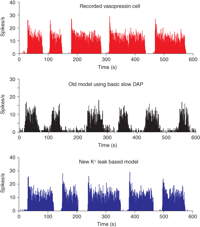
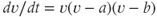
Figure 5.9 The phasic cell and the old and new model. The top panel shows the target phasic pattern, as in Figure 5.1. The old model extends the oxytocin cell model by adding a fast DAP, and a simple dynorphin opposed slow DAP. It produces bursts, but without proper silent periods, or the sharp transitions observed in vivo (parameters in Table 5.3). The new model uses an improved form, replacing the slow DAP with a K+ leak current based mechanism, combining the action opposing action of dynorphin and Ca2+ (parameters in Table 5.4).
However, bursts with this model still do not show the sharp transitions of phasic activity observed in vivo, and the silent period is not particularly silent; this can be improved by using a very hyperpolarized resting potential, but this affects the patterning of intraburst spiking. In a model that is subject to sustained synaptic input and that generates depolarization, it is actually more difficult to explain the silent periods than to explain the burst activity.

Full access? Get Clinical Tree


