(18.1)
where d is the fraction size, D is the total delivered dose, t is the difference between the total treatment time (T) and the lag period before accelerated clonogen repopulation begins (T K), and T pot is the potential doubling time of the cells. The ratio ln 2/T pot is referred to as the repopulation parameter. Several variations of this model have been proposed including a Poisson-based [20] and a birth–death model [21]. Among the most commonly used LQ-based TCP models [22] is:

(18.2)
18.3 Machine Learning for TCP Modeling
Machine learning allows for exploiting nonlinear patterns in the data that may not be directly tractable from using analytical or phenomenological models. There are several steps into development of a TCP model using machine learning as shown in the examples below using dosimetric, clinical, imaging, and biological data in lung cancer.
18.4 Example 1: Dosimetric and Clinical Variables
18.4.1 Data Set
A set of 56 patients diagnosed with non-small cell lung cancer (NSCLC) and who have discrete primary lesions, complete dosimetric archives, and follow-up information for the endpoint of local control (22 locally failed cases) is used. The patients were treated with three-dimensional conformal radiation therapy (3D-CRT) with a median prescription dose of 70 Gy (60–84 Gy). The dose distributions were corrected for heterogeneity using Monte Carlo simulations [24]. The clinical data included age, gender, performance status, weight loss, smoking, histology, neoadjuvant and concurrent chemotherapy, stage, number of fractions, tumor elapsed time, tumor volume, and prescription dose. Treatment planning data were de-archived and potential dose–volume histogram (DVH) prognostic metrics were extracted using CERR [25]. These metrics included Vx (percentage volume receiving at least x Gy), where x was varied from 60 to 80 Gy in steps of 5 Gy, mean dose, minimum and maximum doses, and center of mass location in the craniocaudal (COMSI) and lateral (COMLAT) directions. This resulted in a set of 23 candidate variables to model TCP. The modeling process using nonlinear statistical learning starts by applying dimensionality reduction technique such as principal component analysis (PCA) to visualize the data in two-dimensional space and assess the separability of low-risk from high-risk patients. Separable cases could be modeled by linear kernels while non-separable cases are modeled by nonlinear kernels that allow for separability of the data but at the expense of increased dimensionality. This step could be preceded by a variable selection process and the generalizability of the model is evaluated using resampling techniques as discussed below [26].
18.4.2 Data Exploration
In Fig. 18.1a, we show a correlation matrix representation of the selected candidate variables with clinical TCP and cross-correlations among themselves using Spearman’s rank correlation coefficient (rs). Note that many DVH-based dosimetric variables are highly cross-correlated, which complicate the analysis of such data. In Fig. 18.2b, we summarize the PCA analysis of this data by projecting it into two-dimensional space for visualization purposes. The plots show that two principal components are able to explain 70 % of the data and reflect a relatively high overlap between patients with and without local control, indicating potential benefit from using nonlinear kernel methods.
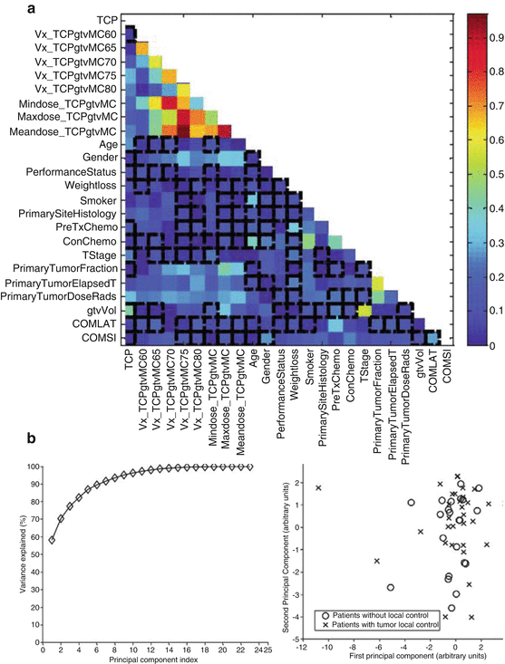
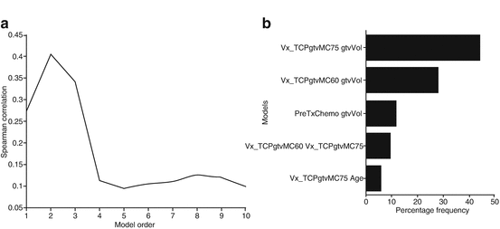

Fig. 18.1
(a) Correlation matrix showing the candidate variable correlations with TCP and among the other candidate variables. (b) Visualization of higher dimensional data by principal component analysis (PCA). Left The variation explanation versus principal component (PC) index. Right The data projection into the first two principal component space. Note the cases overlap

Fig. 18.2
TCP model building using logistic regression. (a) Model order selection using LOO-CV. (b) Model parameters estimation by frequency selection on bootstrap samples
18.4.3 Logistic Regression Modeling Example
The multimetric model building using logistic regression is performed using a two-step procedure to estimate model order and parameters. In each step, a sequential forward selection strategy is used to build the model by selecting the next candidate variable from the available pool (23 variables in our case) based on increased significance using Wald’s statistics [12]. In Fig. 18.2a, we show the model order selection using the LOO-CV procedure. It is noticed that a model order of two parameters provides the best predictive power with Spearman rank correction coefficient (rs = 0.4). In Fig. 18.2b, we show the optimal model parameters’ selection frequency on bootstrap resampling (280 samples were generated in this case). A model consisting of GTV volume (β = −0.029, p = 0.006) and GTV V75 (β = +2.24, p = 0.016) had the highest selection frequency (45 % of the time). The model suggests that increase in tumor volume would lead to failure, as one would expect due to increase in the number of clonogens in larger tumor volumes. The V75 metric is related to dose coverage of the tumor, where it is noticed that patients who had less than 20 % of their tumor covered by 75 Gy were at higher risk of failure. However, a drawback of this logistic regression approach is that it does not automatically account for possible interactions between these metrics nor does it account for higher-order nonlinearities.
18.4.4 Kernel-Based Modeling Example
To account for potential nonlinear interactions as revealed by the PCA, we will apply kernel-based methods using support vector machines (SVM). Moreover, we will use the same variables selected by the logistic regression approach. We have demonstrated recently that such selection is more robust than other competitive techniques such as the recursive feature elimination (RFE) method used in microarray analysis. In this case, a vector of explored variables is generated by concatenation. The variables are normalized using the z-scoring approach to have a zero mean and unity variance [27]. We experimented with different kernel forms; best results are shown for the radial basis function (RBF) in Fig. 18.3a. The figure shows that the optimal kernel parameters are obtained with an RBF width σ = 2 and regularization parameter C = 10,000. This resulted in a predictive power on LOO-CV rs = 0.68, which represents 70 % improvement over the logistic regression analysis results. This improvement could be further explained by examining Fig. 18.3b, which shows how the RBF kernel tessellated the variable space nonlinearly into different regions of high and low risks of local failure. Four regions are shown in the figure representing high/low risks of local failure with high/low confidence levels, respectively. Note that cases falling within the classification margin have low confidence prediction power and represent intermediate-risk patients, i.e., patients with “border-like” characteristics that could belong to either risk group [26].
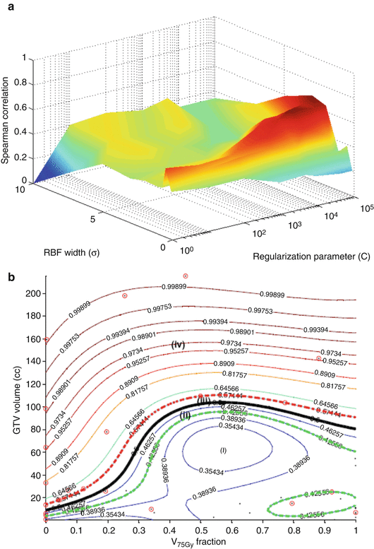

Fig. 18.3
Kernel-based modeling of TCP in lung cancer using the GTV volume and V75 with support vector machine (SVM) and a radial basis function (RBF) kernel. Scatter plot of patient data (black dots) being superimposed with failure cases represented with red circles. (a) Kernel parameter selection on LOO-CV with peak predictive power attained at σ = 2 and C = 10,000. (b) Plot of the kernel-based local failure (1-TCP) nonlinear prediction model with four different risk regions: (i) area of low-risk patients with high confidence prediction level, (ii) area of low-risk patients with lower confidence prediction level, (iii) area of high-risk patients with lower confidence prediction level, and (iv) area of high-risk patients with high confidence prediction level. Note that patients within the “margin” (cases ii and iii) represent intermediate-risk patients, which have border characteristics that could belong to either risk group
18.4.5 Comparison with Other Known Models
For comparison purposes with mechanistic TCP models, we chose the Poisson-based TCP model and the cell kill equivalent uniform dose (cEUD) model. The Poisson-based TCP parameters for NSCLC were selected according to Willner et al. work [28], in which the sensitivity to dose per fraction (α/β = 10 Gy), dose for 50 % control rate (D50 = 74.5 Gy), and the slope of the sigmoid-shaped dose–response at D50 (γ50 = 3.4). The resulting correlation of this model was rs = 0.33. Using D50 = 84.5 and γ50 = 1 .5 [29, 30] yielded an rs = 0.33 also. For the cEUD model, we selected the survival fraction at 2 Gy (SF2 = 0.56) according to Brodin et al. [31]. The resulting correlation in this case was rs = 0.17. A summary plot of the different methods predictions as a function of binned patients into equal groups is shown in Fig. 18.4. It is observed that the best performance was achieved by the nonlinear (SVM-RBF). This is particularly observed for predicting patients who are at high risk of local failure.
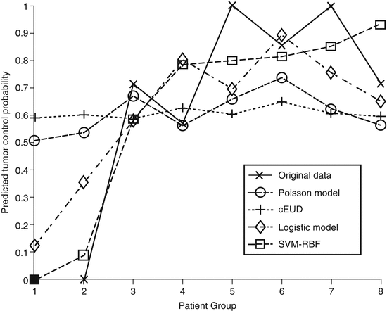

Fig. 18.4
A TCP comparison plot of different models as a function of patients being binned into equal groups using the model with highest predictive power (SVM-RBF). The SVM-RBF is compared to Poisson-based TCP, cEUD, and best two-parameter logistic model. It is noted that prediction of low-risk (high-control) patients is quite similar; however, the SVM-RBF provides a significant superior performance in predicting high-risk (low-control) patients
18.5 Use of Imaging Features
Pretreatment or posttreatment information from anatomical or functional/molecular imaging could be used to monitor and predict treatment outcomes in radiotherapy. For instance, changes in tumor volume on computed tomography (CT) have been used to predict radiotherapy response in NSCLC patients [32, 33]. On the other hand, functional/molecular imaging, in particular positron emission tomography (PET) with fluorodeoxyglucose (FDG), has received special attention as a potential prognostic factor for predicting radiotherapy efficacy [34–37]. For instance, high FDG-PET intensity has been shown to correlate with poor local control in lung cancer [38–41]. In our previous work, new features based on image morphology, intensity, and texture/roughness can provide a more complete characterization of uptake heterogeneity [37]. Recently, we have shown that in addition to PET features, CT-derived features (from the gross target volume) may also improve prediction of local tumor response as shown in Fig. 18.5 [42].
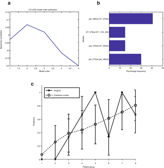

Fig. 18.5


Multimetric modeling of locoregional failure from PET/CT features. (a) Model order selection using leave-one-out cross-validation. (b) Most frequent model selection using bootstrap analysis. (c) Plot of locoregional failure probability as a function of patients binned into equal-size groups showing the model prediction and the original data
Stay updated, free articles. Join our Telegram channel

Full access? Get Clinical Tree


