where α (1/Gy) and β (1/Gy2) are parameters that determine the shape of the curve. Indeed, a vast literature exists on the mechanistic and empirical history of this famous equation, and entire books have been written about the mathematics of radiobiology (Hall and Giaccia 2011; Dale and Jones 2007).
To underscore the contemporary relevance of mathematical modeling in the spatial and biological optimization of RT, a point-counterpoint piece published in Medical Physics in 2016 (Kim et al. 2016) contends that, “With newly available tools such as functional imaging and mathematical models to better estimate the patient-specific, radiobiological parameters … spatiotemporal optimization will enhance current efforts to find more effective treatment schedules to improve patient outcome.” The argument against the contention only questions the degree of the potential gains with RT optimization alone; suggests that increased use of RT + chemotherapy or RT + radiosensitizers will achieve larger gains; and laments that progress will take at least five years, partially due to the need for validated mathematical models. Both of these arguments are likely true, and both are actually encouraging for the broader view on the role of mathematical modeling in the optimization of RT-based therapies.
Similarly, several authors have previously discussed the clinical and translational relevance of mathematical models to predict tumor growth and response to RT (Yankeelov et al. 2013; Jackson et al. 2014; Baldock et al. 2013; Gallasch et al. 2013). Mathematical models can inform clinical practice in a number of ways: via patient-specific models of tumor growth and response to RT, by guiding the design of preclinical studies to predict radiation sensitivity, by helping select patients for definitive clinical trials on these mathematically-driven treatment enhancements, and ultimately by optimizing radiation dose and treatment planning. The challenges involved with the inter-disciplinary, iterative cycle between development, testing, and application of mathematical models in collaboration with clinicians and experimental biologists, as well as some recent successful examples, are summarized by Michor and Beal (2015).
2 Illustrative Mathematical Models of Cellular- and Tissue-Scale Responses to Radiation
Here we summarize a few tenets and principles of mathematical modeling in radiation oncology. As the intended audience of this review is the clinical radiation oncologist, we omit gratuitous mathematical detail in favor of a more heuristic view, and point the reader to excellent reviews as well as more technical literature for the mathematical details of the models. A schematic overview of mathematical modeling in RT is provided in Fig. 1.
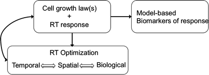

Fig. 1
Mathematical models provide a path to precision medicine in radiation oncology through prediction and optimization of response to RT based on an individual patient’s tumor biology. Mathematical models are used to predict cell growth and response to RT, to optimize RT dose, and may also provide biomarkers (metrics) that can be used to identify and predict which patients will respond to a given treatment course
Ultimately, a mathematical model aims to predict response to RT, although the endpoints defining a response may vary from shrinkage in tumor size, to surviving fraction of cells (Powathil et al. 2013; Prokopiou et al. 2015; Rockne et al. 2010), to predictions of overall survival and similar clinical endpoints (Zaw et al. 2014; Baldock et al. 2012). In this section, we survey increasingly complex mathematical models of cellular- and tissue-scale tumor growth and response to RT.
Starting with simple dose-equivalence and dose-response models, the biologically effective dose (BED) and similar concepts date back to the earliest forms of ionizing radiation as a treatment for human maladies. Since then, many mathematical formalisms have been proposed to incorporate additional variables (e.g., cell proliferation, DNA damage, repair, and ultimately the surviving fraction of cells) into a variety of radiation doses and energies. Mathematically, these models tend to take the form of ordinary differential equations that describe the rate of change of the tumor population with and without the effects of radiation, which is described as a negative rate of change. Tumor doubling time (td), which is nominally incorporated in the basic LQ model, is a simplistic interpretation of these concepts. The concept of tumor control, and tumor control probability (TCP), given by
 where N is the number of tumor cells, and SF is the surviving fraction, can be used as a simple measure to evaluate the success of a given treatment protocol. Several different formalisms for evaluating TCP have been proposed, which vary in complexity (Gong et al. 2013).

2.1 Tumor Growth Laws
Tumor cell growth laws often come in variations of a few archetypes: exponential growth, volume-limited logistic growth, or growth rate-limited Gompertzian growth. One or more of these growth models are then paired with mathematical models of response to RT, often based on the LQ model; this subject is thoroughly reviewed with mathematical details by Enderling et al. (2010) and O’Rourke et al. (2009). However, it is debated whether the LQ model is appropriate to describe biological responses to high dose per fraction treatments such as radiosurgery, which can involve doses of up to 20 Gy in a single fraction (Kirkpatrick et al. 2009). As a result, more complex mathematical models have been proposed to account for potentially different biological effects of high dose RT, which include mechanisms of DNA damage and repair kinetics (Siam et al. 2016; Tariq et al. 2015; Watanabe et al. 2016).
2.2 More Complex Multiscale Models
Mathematical models can also include multiple scales in space and time. Models that include cell motility, surrounding tissues, and spatial variations in radiation dose, for example, often take the form of partial differential equations (Stamatakos et al. 2006; Ribba et al. 2006; Powathil et al. 2007) or agent-based models (Scott et al. 2016). These spatial models may include biophysical forces between the tumor and the surrounding tissue, which may influence cell response to radiation-induced damage (Angeli and Stylianopoulos 2016). In addition, environmental factors that influence response to RT can be included in mathematical models. For example, hypoxia, or lack of oxygen, mediates production of DNA-damaging oxygen free radical species in response to radiation. Thus, changes in the spatial and temporal distribution of hypoxia within the tissue can affect cell kill. A number of groups have incorporated hypoxia into both tumor growth and response to RT models (Scott et al. 2016; Malinen et al. 2006; Titz and Jeraj 2008; Jeong et al. 2013; Rockne et al. 2015).
2.3 Pros and Cons of Model Complexity
Although a variety of mathematical models of tumor growth and response to RT exist, a philosophical argument must be considered regarding model complexity and the ability of the model to be parameterized, and to reasonably provide predictive value. In this way, the number of parameters, often a measure of a model’s complexity, is weighed relative to the biological assumptions in the model. For instance, models that include environmental factors such as hypoxia tend to be more complex, and involve more equations, more parameters, and more specific assumptions. In contrast, simpler models often involve fewer, but broader, assumptions, and also fewer parameters. Such models can more easily be adapted to individual patient data to make patient-specific models and predictions.
Considering the spectrum of model complexity, along with ease-of-use, and evaluating potential utility in the clinical setting, is a challenge for several reasons. One reason is that complex models are difficult to communicate to non-mathematicians, and are difficult to interpret, even by the mathematicians who craft them. An additional concern is that metrics used for decision-making derived from complex models may be sensitive to small changes in the model’s parameters, making the decision-making less robust to variations seen in real data. Finally, more complicated models are not necessarily more effective, as many complicated models make predictions similar to simple models, as shown by Gong et al. (2013).
Simple models, on the other hand, may not include mechanisms or biological detail satisfying to a biologist or clinician, and may miss important features that determine optimal treatment planning, but have the value of being relatively clear to communicate. This highlights just some of the hurdles that support the earlier contention that, even with the ongoing effort in the field, definitive studies on the use of these more complex mathematical models that customize RT to the patient and the patient’s disease will most likely not be completed within five years.
3 Personalized Models
Patient-specific mathematical models provide one means of approaching the ultimate goal of precision medicine: to tailor the treatment to the individual patient’s disease. Baldock et al. provide a roadmap for translating patient-specific models into precision medicine (Baldock et al. 2013), and describe the application of mathematical models to address a variety of clinical questions, such as prediction of surgical outcomes and response to RT. These applications of patient-specific mathematical modeling are connected to the goals of precision medicine, in that biological characteristics of each patient’s disease are incorporated into a tailor-made mathematical model that can provide predictions of response for that individual patient. These predictions can then be used to both better select patients for clinical trials of novel approaches and define cases in which treatment can be rationally modified. In settings with a high cure rate, such as head and neck sarcoma, conventional RT approaches with mathematical models may have a limited value. However, in settings in which the response rate is low or highly variable, personalized mathematical models may provide a means to select patients for a clinical trial, or perhaps modify the treatment plan.
Several methods have been proposed to personalize mathematical models for individual patients. The most common approach is to fit a model to patient data by adjusting parameters in a fixed model. This can be done through a variety of methods, with Bayesian inference (Hawkins-Daarud et al. 2013; Tariq et al. 2016) and model-data fitting procedures (Rockne et al. 2010; Hathout et al. 2015a; Colombo et al. 2015) being two of the most prevalent methods in recent years. For model-fitting algorithms, the most common forms of input are tumor volume and shape characteristics obtained from magnetic resonance imaging (MRI) (Rockne et al. 2010; Neal et al. 2013; Hathout et al. 2015b), positron emission tomography (PET) (Rockne et al. 2015; Mz et al. 2013), or computed tomography (CT) (Prokopiou et al. 2015; Belfatto et al. 2015). These approaches estimate parameters in the model(s) that correspond to biological characteristics of the tumor, such as cell doubling time, proliferation rate, and rate of migration into the surrounding tissue.
3.1 Proliferation Saturation Index
Prokopiou et al. (2015) have derived a proliferation saturation index (PSI) from a model of tumor cell growth and response to RT with a simple logistic growth law, given by
 where PSI is the tumor volume-to-carrying capacity ratio (V/K). Radiation response is determined by the LQ model and is given by


The authors provide a novel perspective on the famous logistic growth equation by using the PSI as a predictive variable for RT response. The patient-specific parameter, PSI, is estimated using regression to fit the logistic growth equation, using data derived from two pre-treatment CT scans. The authors show that PSI correlates with RT response, defined by the post-treatment CT scan, and use their model to simulate different treatment and fractionation schemes that show improved response and tumor control for the individual patient.
3.2 Estimating Radiobiological Parameters
A popular formalism for modeling tumor proliferation, migration, and response to RT takes the form of a partial differential equation to incorporate spatial and temporal variations in the tumor growth, radiation delivery, and radiation response. Although many other models have been proposed, the following model for glioblastoma response to RT provides a means to estimate the LQ radiobiological parameters for individual patients using tumor volume data before and after treatment (Rockne et al. 2009, 2010). The model is given by
 where the tumor cell density (c(x, t)) is a function of space (x) and time (t), and its rate of change is determined by random Brownian motion in the form of diffusion, with migration rate Φ, and logistic growth with proliferation rate ρ. The parameters of this model can be estimated using serial MRI data prior to treatment (Rockne et al. 2010). The delivery and response to RT is given by the term R(c, t, D), where D is the dose of radiation, and the instantaneous rate of cell kill from radiation is given by (1 − SF), where SF is the surviving fraction determined by the LQ model, as follows:


Holding the α/β ratio constant, this model may be fitted to tumor volume data to obtain patient-specific estimates of radiation sensitivity, quantified by the LQ parameter α, as we have shown in Rockne et al. (2010). Moreover, a positive correlation is found between the tumor proliferation rate and radiation sensitivity. This correlation provides a prediction of response to RT, since the proliferation rate is calculated with pre-treatment imaging data. This approach enables patient-specific simulations of alternate RT plans that use response to conventional treatment as a reference. Although approaches for estimating patient-specific radiobiological parameters from imaging data have been criticized for being ill-posed (Chvetsov et al. 2015), the technique is formally no different than a parameter estimation algorithm. In this case, the patient-specific radiobiological parameter α may be used to identify patients likely to respond to RT and that may also be validated in observational studies, used in optimization algorithms, and used to select patients for clinical trials, all of which can potentially lead to advances in patient outcome.
4 Treatment Optimization
A logical extension of personalized models of tumor growth and response to RT is optimization of treatment for the patient. Model-based biomarkers may be included along with dose constraints as inputs to algorithms that can maximize response while minimizing dose to normal tissue. Despite the development of patient-specific cell lines and preclinical animal studies, translating in vitro cell survival curves parameterized by the LQ or other mathematical models into optimized RT for individual patients remains problematic. To overcome this, recent literature in radiation treatment optimization has focused on themes of optimizing radiation dose distributions, biological response, and target volume delineation.
4.1 Spatial Dose and Fractionation Optimization
In order to optimize radiation dose, in addition to existing clinical treatment planning which conforms the dose to the target volume, organs at risk (OARs) are identified, and dose to normal tissue is constrained. These spatial optimizations are incremental advances over the routine conformal or intensity-modulated radiation therapy (IMRT) practices currently standard in clinical radiation oncology. Multi-objective evolutionary algorithms (MOEAs) take OARs and normal tissue doses as constraints into the clinical problem of dosimetry, while also maximizing TCP to the target volume (Holdsworth et al. 2010; Kim et al. 2012). These algorithms can also include objectives to be maximized, such as tumor size or cell kill (Corwin et al. 2013). Groups have already demonstrated the feasibility of implementing spatial optimization of dose using multi-objective evolutionary algorithm methods into a clinical workflow (Kim et al. 2015; Smith et al. 2016). The incorporation of patient-specific tumor growth and response models into this paradigm is a reasonable goal.
The temporal optimization of RT through fractionation attempts to minimize normal tissue complications and incorporate cell repair from radiation damage into the mathematical models. Fractionation schemes are often compared with dose equivalence calculations that are typically based upon the LQ model (Holloway and Dale 2013). In addition to BED- and LQ-based calculations of dose equivalence, tumor growth models can be incorporated into optimization algorithms that explicitly model changes in tumor volume. This enables adaptive fractionation schemes that are tailored to the response of the tumor (Unkelbach et al. 2014b) or that include dose to multiple normal tissues (Saberian et al. 2016). Badri et al. (2015) have taken this approach to apply a mathematical optimization for glioblastoma and demonstrate improved tumor control after mathematical model-predicted improved response to an alternative treatment regime in which the treatment fractions were temporally optimized to minimize toxicity to early and late responding normal tissues. The treatment plans suggested by Badri et al. were also constrained by the 8 a.m.–5 p.m. clinical workday, to provide a practical dosing schedule that could be performed in the clinic.
Stay updated, free articles. Join our Telegram channel

Full access? Get Clinical Tree


