Chapter 6
Modeling Endocrine Cell Network Topology
David J. Hodson, Francois Molino and Patrice Mollard
CNRS, UMR-5203, Institut de Génomique Fonctionnelle, F-34000 Montpellier, France
INSERM, U661, F-34000 Montpellier, France
Universités de Montpellier 1 & 2, UMR-5203, F-34000 Montpellier, France
Department of Medicine, Section of Cell Biology and Functional Genomics, Imperial College London, Imperial Centre for Translational and Experimental Medicine, Hammersmith Hospital, Du Cane Road, London W12 0NN, UK
University Montpellier 2, Centre National de la Recherche Scientifique, Unité Mixte de Recherche 5221, Laboratoire Charles Coulomb, F-34095 Montpellier, France
6.1 Introduction
6.1.1 Overview of pituitary networks
A long-standing conundrum in endocrinology has been the observation that two-dimensional culture of cells results in impaired hormone secretion compared with measures taken from the intact pituitary gland. From this, an important role of tissue context for endocrine cell function has been inferred. However, until recently, the in situ assessment of endocrine cell function has been restricted to immunohistochemistry alongside functional assays that rely on the crude identification of cells using nonspecific secretagogues. To circumvent these problems, a range of transgenic animals with cell-specific tags have been created, opening up the possibility of mapping and recording the structure and function of cells within their native environment using two-photon and allied imaging approaches. By applying these methods to intact tissue, we have so far provided evidence for network organization of four endocrine (gonadotrope, corticotrope, lactotrope, and somatotrope) (Bonnefont et al., 2005; Budry et al., 2011; Hodson et al., 2012b) and two nonendocrine ( folliculostellate, sex determining region Y-box 2 (SRY2 or SOX2)) (Fauquier et al., 2001; Mollard et al., 2012) pituitary cell populations, with consequences for hormone release (Figure 6.1). In this chapter, we will concentrate on the experimental techniques and the data analysis tools available to investigate functional network organization in endocrine tissues.
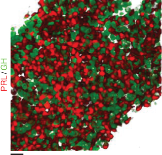
Figure 6.1 High-resolution snapshot of two intermingled pituitary networks (PRL, prolactin; GH, growth hormone) (scale bar = 20  m).
m).
6.1.2 Free cytosolic calcium as a determinant of endocrine network dynamics
To determine a functional network, a population measure of cell activity is required. In large organs, such as the brain, functional magnetic resonance imaging ( fMRI) signals tend to be used to map interactions between distant areas (Bullmore and Sporns, 2009), whereas calcium (Ca2+)-imaging is used to monitor the contribution of individual neurons to the function of discrete neural circuits (e.g., hippocampus) (Peterlin et al., 2000). As the pituitary is a small organ – the size of a pea in humans – large swathes can easily be mapped using the latter approach. Moreover, basal- and secretagogue-stimulated hormone release from most neuroendocrine cells depends on action potential-driven extracellular Ca2+-entry through voltage-gated ion channels (a notable exception being mammalian gonadotropes) (Mollard and Schlegel, 1996; Schlegel et al., 1987; Stojilkovic et al., 2005). Thus, simultaneous assessment of cytosolic free Ca2+ from hundreds of individual endocrine cells allows the activity dynamics underlying hormone secretion to be reasonably estimated. This technique has been widely used in assessing network organization in discrete brain regions.
6.1.3 Problem: defining contributions of endocrine cell networks to hormone release
Decoding the complex network dynamics underlying hormone release is challenging because of our limited knowledge about the nature, strength, extent, and rapidity of cell–cell communication. For example, paracrine couplings mediated by readily diffusible molecules will be subject to different temporal/spatial limitations compared to those that rely on next-neighbor gap junction linkages. Indeed, both exist inside the pituitary, but their exact details remain largely obscure (reviewed in (Hodson et al., 2012aa)). Are the coupling mechanisms of short- or long range? Do they necessitate precise orchestration of cell activity? Are cell–cell communications predominantly homo- or hetero-typic? Consequently, the investigation of structural and functional endocrine cell connectivity is necessarily statistical and descriptive.
The following sections will describe how the mathematical language of graph theory can be used to analyze correlations in position and activity, providing information about the physiologically relevant cell–cell interactions which may contribute to hormone secretion from the pituitary. These tools will then be used in a worked example to analyze spontaneous activity of a pituitary endocrine cell population in situ.
6.2 Networks
6.2.1 Network science
A branch of statistical physics has emerged in recent years to probe the characteristics of complex systems. Relying principally on graph theory, algorithms have been developed to identify the various components of networks, and derive a better understanding of the interactions that occur across multiple scales (μm; seconds to years) to generate complex behavior. Such analyses have deepened our understanding of how network topology permeates seemingly complex scenarios ranging from scientific publishing (e.g., a few influential authors are responsible for the majority of citations) (Price, 1965) to the world wide web (e.g., just a few websites are referred to in the majority of hyperlinks) (Barabási and Albert, 1999) to biology (e.g., protein–protein networks where some key targets such as p53 have wide-ranging effects by virtue of their multiple interactions) (Barabási and Oltvai, 2004). A critical aspect of understanding networks is borne from the observation that, although the constituents can be different (people versus cells) the resultant behaviors/topologies are highly conserved (e.g., random, scale-free and small world).
6.2.2 Network criteria
For a system to behave as a complex biological system, a set of criteria, as adapted from Alon (Alon, 2003), must be fulfilled (see Text Box 6.1).
6.2.3 Network jargon
- Nodes and edges: A network is constructed of nodes connected by edges. In biology, the nature of nodes can vary from individual cells to distinct tissue regions responsible for a particular function.
- Node degree (k): The number of edges emanating from each node. The population degree distribution probability largely determines network topology.
- Node association: A measure of similarity between nodes which determines node degree. This is normally based upon statistical observations of nonrandom behavior such as cell–cell correlation measures.
- Adjacency matrix: Usually a binary table (i.e., “0” or “1”) specifying whether cell 1 is statistically connected/associated to cell 2,…,x. It contains all possible pairwise permutations and allows the calculation of the node degree.
- Network topology: A characteristic description of the network structure drawn from the degree distribution in combination with various other network measures (see network jargon heading).
- Undirected network: No inference is made about the line origins, that is, both nodes are considered to potentially give rise to the interaction.
- Directed network: Lines originate from a specified node. Requires statistical measures of association which can take into account directionality, for example, Granger causality.
- Node association: A measure of similarity between nodes which determines node degree. This is normally based upon statistical observations of nonrandom behavior such as cell–cell correlation measures.
6.2.4 Network metrics
Quantitative analysis of network topology is critical for a better understanding of how functional connectivity influences network performance. For example, do just a few endocrine cells possess most of the edges, thus acting as hubs, or do all cells contribute equally to network architecture? What are the consequences of this for cell–cell communications, robustness in the face of insults, and downstream outputs, such as hormone secretion and transcription? To aid this, some common metrics are listed in the following with explanations of what their values mean. The necessary input data are derived from the correlation matrix and Euclidean distances (see later for how to derive this information).
- Degree distribution (P(k)): The proportion of nodes in the network which possess degree (k). It is otherwise known as the probability distribution of degrees across the population P(k). The value can be derived from summing the columns of the correlation matrix. Cells with the maximum k-value are considered to possess 100% of the connections. The degree distribution is an important indicator of network topology and geometry. For example, if the distribution obeys a power law, then the network is scalefree, i.e., a hub and spoke architecture. Conversely, if P(k) follows a Poisson or Gaussian distribution, then the network is random, that is, all nodes have identical degrees (or edge number).
Average path length (L): The shortest path between two nodes, averaged for all pairwise combinations, is determined by the following formula:
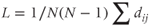
where N is the total number of nodes, and
 is the shortest distance between nodes i and j (summed over all possible node pairs).
In general, the shorter the average path length, the more efficient the information transfer through the network.
Clustering coefficient (C): The number of neighboring edges hosted by a node i as a function of total possible edges (ranging from 0 to 1) and can be calculated using:
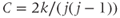
where j is the number of neighboring nodes and k is the number of edges with all neighbors (i.e., degree). The network clustering coefficient is simply the average for all nodes in the population.
High values indicate increased local connectedness with neighbors, streamlining communications due to a tendency toward decreased path length.
Degree centrality (D): A measure of how connected a node’s neighbors are. Degree D centrality of a given node i can be summarized by the following:

where
 if an edge exists between node i and j.
Nodes with high centrality have neighbors with low degree and, thus, act as relays for information flow, minimizing average path length.
- Closeness centrality (CC): The sum of the inverses of the distances between a node and all other nodes:
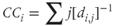
where i is the node under examination and
 is the shortest distance between nodes i and j. Information transfer is most efficient if routed through a central node that is close to all other nodes.
6.2.5 Network topologies
- Random: For a total of n nodes, the probability P that an edge (i,j) exists for all i, j is equal and is denoted by the random graph process G(n,P). That is, all nodes have the same chance of being connected, and the resulting degree distribution is binomial/Poisson (Figure 6.2a).
- Pros:
- Short average path length between any two nodes ensures efficient parallel communication.
- Can maintain function in the face of a targeted insult, since information will be re-routed via other equally connected nodes.
- Short average path length between any two nodes ensures efficient parallel communication.
- Cons:
- Large wiring costs.
- Random and targeted attack will equally disrupt network function, since all nodes contribute to communications.
- Large wiring costs.
- Scale-free: The k degree distribution follows a power law and
 . Scale-free networks are characterized by a “hub and spoke” arrangement whereby a few nodes possess disproportionately many connections. They are ubiquitous throughout science and engineering (e.g., scientific citations, social networks and neural networks possess scale-free topology) (Figure 6.2B).
- Pros:
- Low wiring costs.
- Distant nodes can be connected via hubs with high centrality/closeness, maintaining a reasonable path length.
- Most nodes have a low degree, rendering the network more resistant to disruption by a random attack.
- Low wiring costs.
- Cons:
- Vulnerable to disintegration following targeted attacks against hubs (i.e., nodes with a high degree).
- Average path length is still longer than in a random network.
- Vulnerable to disintegration following targeted attacks against hubs (i.e., nodes with a high degree).
- Small world: These are scale-free networks, with
 and high clustering and assortativity indices. Since the distance d between two edges increases logarithmically with node number (
 ), subnetworks or cliques tend to be formed and most nodes are linked via common neighbours. Small worldness is best epitomized by the six degrees of separation concept (i.e., any two people can always be linked via six contacts) (Figure 6.2C).
- Pros:
- A high clustering coefficient result in a lattice-like structure but with random graph-like path lengths.
- Increased robustness to network perturbation.
- A high clustering coefficient result in a lattice-like structure but with random graph-like path lengths.
- Cons:
- As for scale-free networks.
- Single-scale: The degree distribution (k) follows
 , where
  is the scaling factor. Single-scale networks are lattice-like and possess pros and cons somewhere between random and scale-free networks. They are observed in the nervous system of lower mammals such as Caenorhabditis elegans (Figure 6.2D).
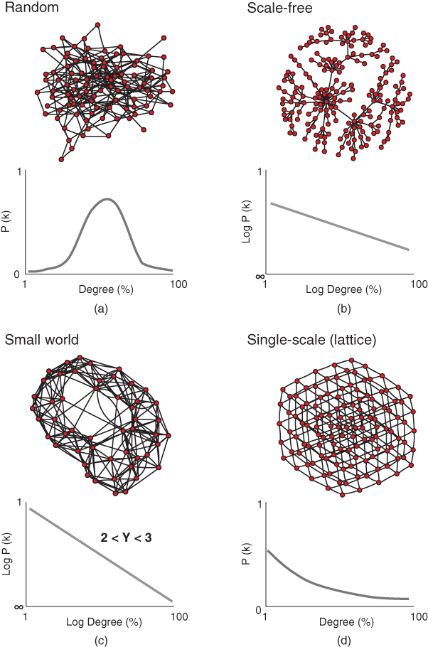
Figure 6.2 Common network topologies based upon degree (or edge number) distribution. (a) A random network (above) has a Gaussian degree distribution (i.e., the proportion of nodes in a network which possess degree k) (below) meaning nodes, on average, possess a similar degree. (b) Degree distribution of a scale-free network (above) follows a power law (below) giving rise to a topology typified by a hub and spoke arrangement. (c) A small-world network (top) has a similar degree distribution probability to a scale-free network, but an exponent value  (below) and high clustering coefficient which results in a shorter average path length. (d) A single-scale network (above) has a lattice like structure determined by its scaling factor
  (below).
6.3 Step-by-step experimental and analytical protocol
6.3.1 Identification of specific cell populations
The use of transgenic animals allows the identification of signals arising from specific pituitary cell populations/lineages. A variety of strains exist which contain fluorophores driven by specific promoters (e.g., prolactin-Discosoma red fluorescent protein (DsRed), luteinizing hormone-Cerulean, growth hormone-enhanced green fluorescent protein (eGFP)). It is important to consider any excitation/emission overlap between the fluorescent tag and Ca2+ indicator when designing imaging protocols.
6.3.2 Pituitary slice preparation
- Prepare bicarbonate buffer (see Table 6.1) and bubble for 10 min with 95% O
 /5% CO
 (! critical: ensure that appropriate local and national ethical approval for animal experimentation is obtained).
- Remove pituitary and embed in 4–5% low melting point agarose diluted in bicarbonate buffer and allow them to solidify on ice.
- Using a scalpel, carefully remove a
 cm2 block of agarose containing the pituitary, secure to the vibratome chuck with superglue and mount in the vibratome bath containing bicarbonate buffer at 4°C (bubbled with 95% O
 /5% CO
 ). Use a fresh blade for each experiment and slice 150–200
  m sections at 60 Hz using the slowest speed setting (! critical: maintain bath at 4°C for optimal slices otherwise agarose can become unstable).
- Use a paintbrush or 5 ml plastic pipette (tip widened with scissors) to retrieve the section. Place on a poly-L-lysine coated (1 mg/ml) coverslip (de-greased with acetone followed by ethanol rinse; size will depend on microscope chamber characteristics) and carefully aspirate excess solution until the section is adherent. Remove excess agarose if still present using two 23G needles (! critical: for best adherence, place 50
 l 1 mg/ml poly-L-lysine in centre of a coverslip and allow to dry at 37°C overnight before attaching pituitary sections).
- Allow sections to recover for 1 h at 37°C, 95% O
 /5% CO
 in bicarbonate buffer.
 - Allow sections to recover for 1 h at 37°C, 95% O
Table 6.1 Bicarbonate buffer constituents
| NaCl | KCl | NaH PO PO | NaHCO | Glucose | CaCl | MgCl |
| (mM) | (mM) | (mM) | (mM) | (mM) | (mM) | (mM) |
| 125 | 2.5 | 1.25 | 26 | 12 | 2 | 1 |
6.3.3 Load with a Ca2+ indicator
- Mix 50
 g fura-2AM with 5
  l DMSO + 10
  l 20% pluronic acid (w/v in DMSO) and sonicate for 3 min. Add 500
  l bicarbonate bufferand sonicate for a further 3 min to disperse micelles. Make up to 2 ml and incubate slice in fura-2-containing solution for 1–2 h at 37°C/5% CO
 . Rinse sections twice with bicarbonate buffer and reincubate for 30 min without fura-2 to allow cleavage and activation of fura-2 intracellular esterases (! critical: do not over-incubate slice to avoid buffering of cytosolic free calcium by fura-2).
- Mount slices on/in microscope chamber and perfuse with bicarbonate buffer at 34–36°C (! critical: ion channel kinetics are temperature-dependent).
- Use a 10–40
 water immersion objective depending on desired size of imaged field. Capture a snapshot of the fluo-tagged cell population under investigation. A
  NA 0.95 water immersion objective allows pituitary slices to be imaged with single-cell resolution whilst retaining a large field of view.
- Proceed to functional multicellular imaging (fMCI).
6.3.4 Functional multicellular calcium imaging (fMCI)
- Perform excitation at 780–800 nm and record emission at 525/50 nm for nonratiometric two-photon imaging of fura-2. Multiphoton microscopy has many advantages over single photon modalities including better depth penetration, less photoxicity and improved axial resolution (see Glossary) (! critical: due to fura-2 excitation above the isosbestic point, increased [Ca2+]
 will present as decreased signal intensity).
- Acquire a three-dimensional reconstruction of the cell population under investigation. This will allow functional connectivity (based on association measures) to be directly correlated with structural connectivity (based on physical linkages) (see later).
- Image fura-2 in the second cell layer. This avoids artifacts due to recording at the cut surface and ensures optimal overlap with the cell fluo-tag. Generally, Ca2+ indicators will penetrate three to four cell layers deep.
- According to the Nyquist sampling theorem, the frame rate should be twice the highest frequency which needs to be resolved for analysis purposes. For example, 1 Hz will be required to detect events at 0.5 Hz. For long-term time lapses (>15 min), reduce laser power, and frame rate at the expense of spatial resolution/image quality (! critical: phototoxicity introduces artefacts into signal analysis).
- Use binning to average intensity for
 pixels if using the an EM-CCD-based system.
Note: Fura-2 is ideal for both one- and two-photon imaging modalities as it possesses nonoverlapping excitation/emissions spectra with commonly used eGFP cell-tags, loads pituitary cells better than equivalent Ca2+ indicators, and possesses a dissociation constant ( 145 nM) compatible with resolution of both spontaneous and secretagogue-driven Ca2+ events in pituitary cells. Since fura-2 can exit cells via chloride channels, “leak resistant” forms are recommended for long time-lapse experiments.
6.3.5 Data extraction
- Export time-lapse sequences as .tif files and open in ImageJ or Fiji (both NIH, USA) (Supplemental Movie 1).
- Obtain an average image of the movie using the Stacks->Z project (mean) function.
- Manually delineate fluo-tagged, fura-2-loaded cells using a region of interest (ROI) accessible from the ROI Manager (Ctrl + T) (Supplemental Figure 6.1 and Supplemental File 1).
- Ensure the correct parameter to be measured is selected in the Set Measurement menu (Analyze-
 Set Measurement-
 Mean Gray Value). On the ROI Manager, toggle Show All and then Multi Measure to extract intensity over time traces for ROI 1….x. Save ROI and intensity-over-time data as .xls/.csv and .zip files, respectively.
6.3.6 Signal processing
Hilbert–Huang empirical mode decomposition (EMD)
This method relies on decomposing nonlinear nonstationary signals into static intrinsic mode functions (IMF) of varying frequencies, which together are responsible for the observed Ca2+ trace. Briefly, the IMFs are extracted using a sifting process of  means determined by a cubic-spline interpolation of the local minima and maxima. The instantaneous frequency of the function
  can then be calculated using a Hilbert transform:
Related posts:
 Modeling the Dynamics of Gonadotropin-Releasing Hormone (GnRH) Secretion in the Course of an Ovarian Cycle
Stay updated, free articles. Join our Telegram channel

Full access? Get Clinical Tree


