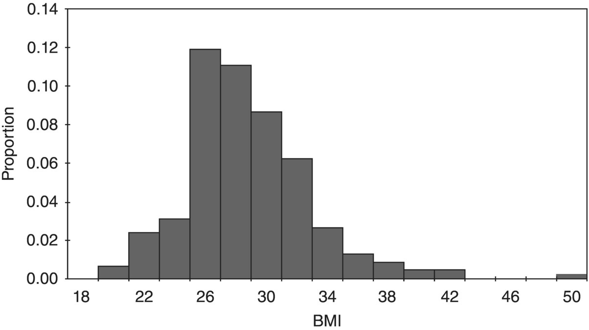
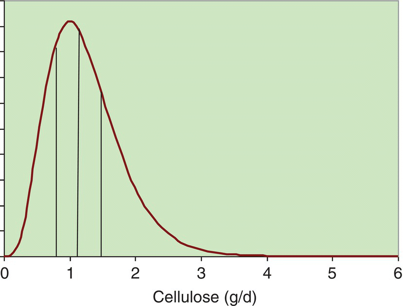
7 Graham Horgan Biomathematics and Statistics Scotland, Rowett Institute of Nutrition and Health, University of Aberdeen This chapter considers the analysis of nutritional data. This includes summarising such data, producing estimates of effects and differences and testing them. It also includes techniques such as principal component analysis that are exploratory, looking for patterns in data. This essentially is statistics, which may be defined as the study of variation. Any collection of nutritional data will certainly show variation. Intake data will vary between subjects (different people eat different things and different amounts) and within subjects (between days, or between baseline and endpoint in an experiment, for example). Food composition will also vary among samples of food items. Our task is to summarise this variability and draw conclusions in its presence. Some of it we will be able to explain. Dietary intakes vary because of a person’s age, gender and weight, for example, and perhaps because of dietary interventions in which they are participating. We try to quantify these effects and test whether we can be sure they are present. Other variations we will be unable to explain. A person will not eat the same things every day. Some of this we can account for (day of the week, activity level and so on, if we have recorded this information), but some of it always remains unaccounted for. Such variation is termed random. Many varied things in people’s day-to-day life (work patterns, social life, the weather) will determine what they eat on different occasions, but since these are unrecorded in our data, we cannot use them to account for the dietary variation. This chapter covers a number of topics in the handling and interpretation of nutritional data. All of them are deserving of a whole chapter, indeed a whole book, in themselves, so we will of necessity have to be brief. Much of what is presented therefore raises issues or questions, rather than offering a detailed discussion of their treatment. Statistics is a scientific discipline. Here we aim to cover the main topics briefly and put them in the context of nutritional data. There are many excellent textbooks that give a good introduction to statistics and those aimed at scientific disciplines allied with nutrition are probably the most useful. We would mention Campbell (1989) and Bland (2000), although there are many others. As may be expected, they vary in style, level of detail and extent of mathematical treatment, and each scientist will need to find one that suits him or her individually. Data variables can be of different types and as this affects how they are handled, it is worth keeping in mind for each variable which type it is. A continuous variable, also known sometimes as a variate or a vector or an interval variable, denotes a quantity of some sort. Larger numbers will denote more of something, and we can speak about differences between values. For values obtained from physical measurements, these variables will usually have units (cm, gram, hour, kg/week and so on). Often a zero value of the variable is possible, and ratios may sensibly be calculated (in which case the term ‘ratio variable’ can be used). The unit scale is usually arbitrary: it is not important whether height is recorded in metres or centimetres, or energy intake in kJ or kcal. A change of scale by multiplying by a constant will not affect a statistical analysis, other than those parts that should scale accordingly. On other occasions variables may be defined that represent quantities that cannot be accessed directly, such as appetite or a psychometric score. These will usually not have units and their values are determined by recording something else (a visual analogue scale, answers in a questionnaire). For most purposes, there are treated in the same way as physical measurements. The other common type of variable is categorical (sometimes termed factor or group), meaning that it records to which of two or more groups an observation belongs. If there are only two groups, the variable is termed binary (e.g. gender, or any yes/no outcome). In a trial where a treatment is offered at different doses, we sometimes regard these as categorical or sometimes as a continuous variable. Finally, an intermediate type of variable is ordinal. In this case the categories follow a natural order. Volunteers may record how much they like a food as ‘not at all’, ‘only a little’, ‘somewhat’, ‘a lot’. There is a natural ordering here, for which we may wish to account in presenting and analysing the data. Opinions are often recorded as the extent of agreement with a statement, and a similar scale results. Observed values are subject to variation, which may either be biological in origin or due to the measurement technique being used. Biological variation is what is generally of interest, whereas measurement variation is typically a nuisance. Measurement variation, sometimes termed technical variation, is the variation that would be observed if several measurements are made on each biological sample, or on an individual person if it is something that is believed to be constant in that individual, at least over the time scale of the measurements. Technical variability can be quite small (e.g. an individual’s height) or substantial, possibly even greater than the biological variation (as in some methods of determining protein expression, for example). If measurement variation is large, and time and costs permit, there may be benefits in doing several repeat measurements on each sample. However, it is important to remember that these are not true replicates, and in any analysis it is the mean of the repeat measurements that should be used. Furthermore, it is almost never a good idea to take repeated technical measurements if it is at the expense of true biological replication. Throughout this chapter it is important to keep in mind that there is some population to which we want the information generated by our research to apply. This may be as wide as humanity in general, or it may be some subset, such as those within a certain age range, or with some specific characteristics (such as obesity). Whatever it may be, we cannot collect data on all of humanity or of the subset. We study a sample. If that sample is representative of a wider population, then we can claim that our conclusions are valid for that population. This representativeness may partly be based on the sample having been selected at random. However, it is often the case in nutritional research that those studied are volunteers or patients, from some geographical region, and their representativeness of any population in particular is an assumption that we need to make, but about which the data cannot inform us. The validity of this generalisation of the results should be discussed when the results are presented. The distribution is a fundamental concept in statistics. It specifies all the details of how some quantity varies. Figure 7.1 shows the observed distribution of body mass index (BMI) in a sample of about 200 adults. It allows us to see the relative proportions of individuals in each range of 2 BMI units (kg/m2). If the sample is representative of some population, we can estimate the probability that an individual in that population will have a BMI in any specified range. The histogram allows us to observe characteristics of the distribution such as skewness (asymmetry), multimodality (more than one peak) and outliers. The most commonly used measure of variability is the standard deviation, defines as the square root of the mean squared deviation of observations about the mean Figure 7.1 Histogram of BMI. The divisor of n-1, termed the degrees of freedom, is used because the deviations are not independent but are constrained to sum to zero. For many purposes in data analysis, it is convenient if random variation has a roughly normal (also termed Gaussian) distribution, one that is symmetrical and bell shaped. Note that it is the distribution of the random unexplained variation that needs to be normal, not necessarily the original values, although the shape of the distribution is usually similar for both. The calculations done in statistical testing, for example, tend to assume this normality. If data depart substantially from this, it may be more reliable to work with a transformed version. There are many possibilities here, but the log transform is by far the most widely used. It tends to make positively skewed distributions more symmetrical, and can be thought of as transforming multiplicative effects and differences into additive ones. If some data values are zero, add a small constant to all values (the smallest non-zero value, for example) before taking logs. If some values are negative, this usually is because they are differences, in which case take logs before calculating differences. A histogram will also alert you to outliers, observations far from the rest of the distribution. These should be checked in case they are errors, or in some way unrepresentative of what you intend to study. However, they cannot be removed without good justification. For example, in Figure 7.1 we might want to check that the BMI observation about 50 is correct. If it had been 5 or 500 we would have been sure that it must have been wrong, and we would either correct it if we could, or omit it if we could not. There are no standard tests to help identify outliers. Scientists must use their own judgement and knowledge of how the data were collected. Sometimes it can be convenient to handle continuous variables by chopping the range of values into intervals to define an ordered categorical variable. The main reason for doing this is convenience. It can be easier to discuss the differences between these categories than to talk about the effects of gradual changes in the continuous variable. In some cases, statistical analysis using the categories is more easily able to account for effects such as non-linearity, which require more care on the continuous scale. Non-linearity occurs when a response does not change at a constant rate as an explanatory variable changes. The definition of the intervals can be done in various ways. Dividing age into decade intervals (20–30, 31–40 etc.) seems natural and easy to remember. BMI is traditionally divided into intervals of < 18, 18–25, 25.1–30 and > 30 as a choice of readily remembered round numbers, and these are used by the World Health Organization. The > 30 range is sometimes further subdivided. Dietary intakes are sometimes split according to whether they meet specified recommendations or not. Splitting the range of values according to the observed distribution is also widely done. This involves choosing dividing points so that the same proportion of observations falls into each interval. The usual choices are three intervals (tertiles) or four (quartiles) or five (quintiles) and occasionally ten (deciles). The advantage of defining categories in this way is that it is objective and frees scientists from the need to choose values themselves. It also ensures an equal number of observations in each category, which is optimal for statistical power. There is a disadvantage to turning a continuous variable into categories, and that is the loss of information that it implies. The usual BMI categories, for example, imply no difference between two individuals with BMIs of 25.5 and 29.5, while the latter is in a different category from someone with a BMI of 30.5. There is also an information loss if the analysis does not account for the ordering of the categories, which very often it does not. In terms of variance information discarded, defining tertiles discards about 21% of the variability, quartiles discards about 14% and quintiles about 10%. This loss of information is illustrated in Figure 7.2. More quantiles result in less loss of information, but more result details have to be presented, and fewer observations per quantile increase the uncertainty about each result. Four quantiles (i.e. quartiles) seem to be the most common choice. Figure 7.2 Example of representing a continuous variable (dietary cellulose) as quartiles. The lowest and particularly the highest contain values with considerable variability. For anything we want the research to tell us – which is typically the mean of a variable, the effect of a treatment, the difference between two population subgroups or the risk of some adverse outcome – we suppose that there is some true value for this quantity. Then there is the value that we estimate in our study. The classic statistical view is that this estimated quantity is subject to variability. If we repeated the whole study, changing nothing but sampling a different but equally representative set of subjects, we would obtain results that were somewhat different. The amount by which an estimated quantity is subject to variability in this way is termed its standard error. We do not need to repeat the study in order to obtain it, as it can be calculated from the information in a single study. The value of a standard error (SE) is that it tells us the reliability of the (single) estimate that we have obtained of some quantity. If the SE is low, then we know that any repeated study would produce a similar estimate, so it must be close to the true value (assuming of course that there is no bias). A standard error can be obtained for any quantity that is calculated from a sample. The most often quoted are the standard error of the mean (SEM = Standard errors and confidence intervals may also be calculated for proportions, such as the proportion of individuals who meet a dietary recommendation. If the proportion in the sample of size n is p, then the SE is Very often the central question in a nutritional investigation is whether or not there is an effect (of one variable on another) or a difference (between two intervention groups) or an association (between two variables). This question is assumed to have an answer ‘yes’ or ‘no’. This is the usual view, although some experts would argue (Nester 1996) that there is always an effect or difference of some sort, even though it may be small. Perhaps we can say that if a difference is small enough that our study cannot even tell whether it is positive or negative, we will regard it as effectively zero. The p-value is based on considering what might be observed if there was no difference or effect or association. Suppose we are comparing an intervention and a control group in a situation where the intervention really has no effect. Ideally, the mean of the outcome of interest would be the same in both groups. In practice, because of random variation, the difference in means will not be exactly zero. Let us call this difference D. The p-value asks the question: ‘How likely are we to observe a value of D as large as this in the absence of any intervention effect?’ The answer is a probability, the p-value. If this is small, we have observed something that is unlikely in the absence of an effect, and so we conclude that there is an effect. Indicating significance using * for p < 0.05, ** for p < 0.01 and *** for p < 0.001 is common. How small does a p-value need to be in order to draw this conclusion? There is no answer to this, and the p-value is a continuous scale of evidence for or against the existence of the effect. There is a convention that 5% is the value below which the evidence is enough. In practice, the p-value calculated should be presented, and the discussion should then proceed to weighing the strength or weakness of the evidence against the consequences of deciding whether or not there is an intervention effect. One final subtlety of the p-value is related to the phrasing in the question: ‘a value of D as large as…’. Conventionally, this is taken to include both positive and negative differences of the specified magnitude, and the test is termed ‘two-sided’. Rarely, we may declare that we are only interested if differences are in one particular direction and a one-sided test results, with half the p-value of the corresponding two-sided version. For example, we could claim that we are only interested in a dietary supplement if it reduces cholesterol, and would declare that it had no effect if evidence pointed to a significant increase. In reality, any such outcome would be noteworthy. Two-sided tests are always recommended. A t-test is the most basic statistical test and is most often used to compare two groups, but it can also compare a single sample against some specified constant. An example is comparing the mean intake against some dietary reference value, a recommended level of intake that many governments and nutritional organisations promote. For example, this might be an Estimated Average Requirement (EAR), published by the Institute of Medicine of the US National Academy of Sciences, expected to satisfy the needs of 50% of the people in that age group and used to assess the contributions of food items to nutritional needs. Also published are Recommended Dietary Allowances (RDA), the daily dietary intake level of a nutrient considered sufficient to meet the requirements of 97.5% of healthy individuals in a group, and this is usually about 20% higher than the EAR. Regression modelling is the most commonly used technique for linking one variable to others. Other techniques such as analysis of variance (see Section 7.4) are also built around regression-type models. In regression we select one specific variable that we regard as the response or outcome, and then study the way in which it depends on other explanatory variables. Depending on the question of interest, things that we measure may play the role of the response or the role of the explanatory variable(s). For example, if we have recorded an individual’s dietary intake of retinol, we might seek to investigate what affects that intake: age, gender, income level, choice of food groups, experimental interventions and so on. Or we may be interested in how retinol intake affects health-related outcomes such as blood pressure or even mortality. In the former case, retinol is the outcome; in the latter, it is blood pressure or whatever. The outcome variable may be of any of the types listed above, as may the explanatory variables. Here we will only consider the simpler cases where the outcome is continuous or binary and the explanatory variables are continuous or categorical or a mixture of these. For a continuous outcome, consider the simplest model where there is one explanatory variable (let us call it X) and the outcome or response variable (call it Y). We then suppose that where A and B are constants that we estimate from the data, and ε denotes random variation, whose variability we also estimate. We assume its mean to be zero. The model is linear in that the effect of changing X is independent of the value of X: an increase of one unit in X is associated with a mean increase of B in Y, regardless of what X is. The constant A is the mean value of Y if X is zero, although as often as not this does not have any practical meaning. Regression can be carried out in almost any statistical software, and will produce various results in the output. These will include: Figure 7.3 shows a plot of bodyfat and triceps skinfold thickness in 20 women (see Neter et al. 1996). We expect these to be related and can see that they are. A plot such as this allows us to judge whether or not a linear model is appropriate. There are ways to test this formally, but that is not discussed here (see Chaterjee and Hadi 2012, §4.7). Examining a plot should always be the first step. A linear model seems a reasonable choice to fit here. However, it is not completely clear which variable should be the explanatory and which the response. If the purpose is to predict body fat (which we want to measure, although this is not easy) from skinfold thickness (which is easy) then body fat should be the response, if the subjects are representative of those for whom we plan to use the prediction. Figure 7.3 shows the output from fitting a linear regression using the open-source R statistical programming language (R Core Team 2012).
Methods of Data Analysis
7.1 Introduction
7.2 The basics of statistics
Types of variables
Biological and measurement variability
Populations and sampling
Distributions, transformations and outliers
 :
:

Quantiles
Standard error and confidence interval
 ) or that of the difference in two means (SED =
  ), but it can also be calculated for a proportion or regression coefficient or anything else calculated from a sample. A common way of presenting the same information is to quote a confidence interval. This is based on the fact that the variability in estimates has a normal distribution, and this distribution encompasses 95% of observations within about 2 standard deviations. So if we quote an interval of plus or minus 2 × SE about an estimate, it will include the true value 95% of the time. In fact, allowing for the SD being estimated rather than known exactly, the correct multiplier is not exactly 2 and depends on the sample size. However, it will not be greatly different from 2, and will be between 1.96 and 2.2 as long as the sample size is at least 10.
 , and the confidence interval is calculated as for the mean.
Tests and p-values
7.3 Regression modelling

Stay updated, free articles. Join our Telegram channel

Full access? Get Clinical Tree


