Methods in Mathematical Modeling for Stem Cells

(18.1)

with the initial condition P(t ₀) = P ₀, where M, δ, γ and θ are parameters. We refer to the model (18.1) as the hyperbolastic ordinary differential equation of type III or H3. This rate of growth is a product of one factor representing the distance of the current population from its limiting value M and a second factor including the intrinsic rate δ, an allometric constant γ, and an additional term θ allowing flexibility in growth rate over time. The solution to the Eq. (18.1) is the function

$P(t)=M-\alpha EXP\left[-\delta {t}^{\gamma }-\mathrm{arcsinh}\left(\theta t\right)\right],$

(18.2)

where

$\alpha =\left(M-{P}_0\right) EXP\left[\delta {t}_0^{\gamma }+\mathrm{arcsinh}\left(\theta {t}_0\right)\right].$

We call the function P(t) of Eq. (18.2) the hyperbolastic growth model of type III or simply H3. If necessary, one can introduce shift or delay parameters in this model. The doubling time t for the model H3, in the case where P ₀ < M/2, is the solution to the equation

$\ln \frac{M-2{P}_0}{\alpha }+\delta {t}^{\gamma }+\mathrm{arcsinh}\left(\theta t\right)=0.$

Here we briefly address the biological meaning associated to the parameters M, δ, γ, and θ. The parameter M has the same units as P(t), the number of stem cells, and it represents the limiting value of the size of the population, or the carrying capacity. The parameter δ corresponds to the intrinsic biological growth rate; however the overall rate of growth is jointly determined by all of the parameters δ, γ, and θ. The units of δ is 1/(time)^γ, which in the cases of this paper is 1/(days)^γ. The parameter γ is known as the allometric constant, and a similar parameter occurs in the Weibull model. This parameter is dimensionless. It is sometimes called a statistical shape parameter. Finally, the parameter θ has units 1/(time), in our case 1/(days), and to more fully describe its biological meaning we rewrite the Eq. (18.2) in the form

$P(t)=M-\frac{\alpha }{\theta t+\sqrt{1+{\left(\theta t\right)}^2}} EXP\left[-\delta {t}^{\gamma}\right].$

For θ = 0, the term in front of the exponential reduces to α, and the model reduces to the Weibull growth model. When θ ≠ 0, the expression $\alpha \left(t,\theta \right)=\frac{\alpha }{\theta t+\sqrt{1+{\left(\theta t\right)}^2}}$ allows this factor to vary with time t, according to this formula and the value of θ. Thus the parameter θ provides variation in the quantity α, which represents a rescaling of the distance between the initial population and the limiting value, allowing adjustment of this growth rate over time. In application of the model a constant value is determined for θ that best represents the growth observed in the data.

In the following paragraphs we apply the hyperbolastic model H3 to some publicly available data on embryonic stem cell growth, found on the NIH website. We consider the cell lines GB01, WA01, and WA07, for which there were 6 days of growth data available, and we display the difference between H3 and the Sherley model, a commonly used model for cellular growth. Although the parameters in the Sherley model represent the dividing time and the proportion of cells actively proliferating, we see that the estimated growth curves for this model do not fit the data points. See Figs. 18.1 to 18.3. In cases like these the parameter estimates cannot really be considered to be representative of the biological data. In contrast, the H3 model provides a very close fit to the data in all three cases. In addition to the significance of the H3 parameters, as presented above, these explicitly defined functions also allow explicit representation of the rate of growth, as given in each of the figures below. We note that this growth rate, and particularly the location of its maximum, can be investigated for the underlying biological significance.

We begin with a statistical assessment of the accuracy of the two models for these data sets. In each case the H3 is considerably more accurate than the Sherley model, and in two of the three cases it is nearly perfect. For the first case of the BG01 cell line, the parameters for the Sherley model are α = 1.000 and DT = 1.770, while the parameters for H3 are M = 762.922, δ = 3.137E-6, γ = 7.990, and θ = 0.051. The H3 model is nearly a perfect fit, with R² of 1.000 and RMS of 8.470, while the Sherley model has R² of 0.966 and RMS of 3096.170. We observe more in Figs. 18.1, 18.2 and 18.3 how H3 really makes a much better representation of the growth curve, capturing the overall shape. In contrast, the Sherley model does not capture the overall shape of the data and can be expected to magnify the errors if time is extended. For the WA01 cell line of Fig. 18.2, the fit of Sherley is a little better, while the fit of H3 is a little worse, although this difference is probably due to the existence of a misplaced point. The Sherley model use parameters of α = 1.000 and DT = 1.770, while the parameters for H3 are M = 10193.018, δ = 4.204E-9, γ = 1.769, and θ = 0.069. With this misplaced point, R² for H3 has decreased to 0.994, with an RMS of 180,819.041. In contrast, Sherley has R² of 0.981 with an RMS of 282,099.496. A case like this is about as close as Sherley can get to H3, due to the placement of the point, as we discuss further below. Nevertheless H3 still provides a considerably better fit, with just over half the RMS or Sherley. The third case of the WA07 cell line returns to a case with points in standard position, and the H3 has a fit with R² = 0.999 and RMS = 17,817.688 with parameters M = 7635.150, δ = 0.003, γ = 4.054, and θ = −0.031, compared to Sherley with R² = 0.955 and RMS = 476,844.808 for parameters α = 0.525 and DT = 0.184. In the Figs. 18.1, 18.2 and 18.3 depicting these models, the dashed curve represents the Sherley model, while the dotted curves represent H3.

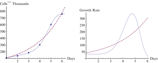
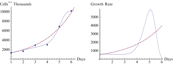
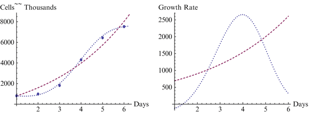
Fig. 18.1

Growth and growth rate for GB01 line, H3 and Sherley models

Fig. 18.2

Growth and growth rate for WA01 line, H3 and Sherley models

Fig. 18.3

Growth and growth rate for WA07 line, H3 and Sherley models

We note that in Fig. 18.1 for the BG01 cell line and Fig. 18.3 for the WA07 cell line the growth curve from H3 captures the overall shape of the data and displays only minimal errors in approximating the points, with each point contacting the curve. This is in marked contrast to the representations by the Sherley model, where the overall shape of the data cannot be represented by the curve and all of the points are at some distance from the curve, yielding considerably more error in approximation. As each of the figures clearly represent self-limiting, or sigmoidal shaped growth, the H3 model clearly better represents the growth, and the increasing growth rate of the Sherley model will lead to even larger errors for extended time.

The case in Fig. 18.2 for growth of the WA01 cell line is interesting because of the unusual pattern in the data for days 3 and 4, where the data shows the number of cells is static, in contrast to the standard pattern of growth. Sherley model is able, by coincidence, to find a close fit to the other data points by nearly neglecting the data point from Day 4. However, clearly this curve still does not represent the overall sigmoidal shape of this or the other data sets. The H3 model cannot attain as high an accuracy as the other cases as the curve straddles the data points for days 2, 3, and 4. But it is still very close, and is clearly the better representation of the two curves, even moreso than can be seen in the differences in R² and RMS. Note that with a slightly lower value on day 3 or a slightly higher value on day 4, Fig. 18.2 would fit the same pattern as Figs. 18.1 and 18.3, and the statistical measures of fit would return to the comparable level.

The above examples of applying the H3 model to represent proliferation of embryonic stem cells are representative of the high level of accuracy found in this model. The papers of Bursac et al. (2006) and Tabatabai et al. (2011b) compare the accuracy of diverse models for the proliferation of the BG01 cell line, demonstrating that H3 indeed provides the best fit, followed closely by the other hyperbolastic models H2 and H1. The paper of Tabatabai et al. (2011b) also demonstrates the accuracy of the hyperbolastic models, particularly H3, in representing the proliferative index for adult stem cells. We assume these models are equally effective in representing proliferation of induced pluripotent stem cells.

We are currently developing the hyperbolastic models H1 to H3 in several further directions. One such direction is the development of robust methods for these hyperbolastic models so they can maintain an accurate representation of the growth curve, even when one or several of the points are displaced. The above discussion allied with the growth curve for the WA01 cell line as depicted in Fig. 18.2 is representative of some of the difficulties that can arise in robustness for such non-linear models, due at least in part to the flexibility in the shape of the curve. In addition we are currently developing these hyperbolastic models for use in longitudinal studies as non-linear hyperbolastic mixed effect models. We also note that a multivariable version of the model already exists and has been applied in Tabatabai et al. (2011b), in Tabatabai et al. (2011a), and in a recent work of the authors modeling phytoplankton growth dynamics. This multivariable version uses a link function and additional parameters to represent the role of additional covariates in accelerating or decelerating the growth rate. One additional topic for continuing development will be in relation between the model parameters and the biological characteristics of the system being modeled. Particularly in cases where these models are used together in a system of differential equations, as in the section on the Integrative Model below, it will be important to tie the model parameters in to the biological characteristics.

Differentiation

Another fundamental property of stem cells is their ability to differentiate into a variety of cell types, as required for use within the organism. The course of differentiation is primarily guided by gene expression and epigenetic regulation, and an important role is also played by intercellular signaling, primarily directed by growth factors and other soluble factors. A more thorough understanding of the means of directing differentiation is desirable and would be beneficial to stem cell therapies. Here we propose use of two mathematical models that can assist in the study of differentiation of stem cells and the role of explanatory variables. The first of these models is a survival model which can be applied to study the time to event in various applications, including survival time, time until maturation, healing time, as well as many others. In the present context we will study time until differentiation of stem cells together with the influence of one or more covariates, such as level of oxygen or differentiating agents, on the differentiation time. One of the main concerns here is a quantitative assessment of the role of such explanatory variables on the differentiation procedure. The key features of the model we use, the hypertabastic survival model introduced in Tabatabai et al. (2007), are the quantification of the roles of one or more covariates and the flexibility of the distribution in assuming various shapes of hazard curves dependent upon the underlying distribution of data.

We begin by defining the hypertabastic distribution function, which is given as follows

$$$ F(t)=\Big\{\begin{array}{ll}1- sech\left\{\alpha \right[1-{t}^{\beta } coth\left({t}^{\beta}\right)\Big]/\beta \Big\}\hfill & t>0\hfill \\ {}0\hfill & t\le 0\hfill \end{array} $$ ” src=”/wp-content/uploads/2017/02/A320614_1_En_18_Chapter_Equd.gif”></DIV></DIV></DIV>The hypertabastic probability density function is given by<br /> <DIV id=Equ3 class=Equation><br /> <DIV class=EquationContent><br /> <DIV class=MediaObject><IMG alt=$ 0\hfill \\ {}0\hfill & t<0\hfill \end{array} $$ " src="/wp-content/uploads/2017/02/A320614_1_En_18_Chapter_Equ3.gif">

(18.3)

where W(t) = α[1 − t ^βcoth(t ^β)]/β, and α, β > 0.

The hypertabastic proportional hazard model has a hazard function of the form

$h\left(t\Big|x,\theta \right)={h}_0(t)g\left(x\Big|\theta \right)$

(18.4)

where h₀ (t) is the baseline hazard function, given by

$\begin{array}{c}{h}_0(t)=\alpha \left[{t}^{2\beta -1} csc{h}^2\right({t}^{\beta}\left)-{t}^{\beta -1} coth\right({t}^{\beta}\left)\right]\\ {}\kern1em tanh\left[W(t)\right].\end{array}$

We will use g(x|θ) = Exp[Σp_k = 1 θ _kx _k]. The x_k represent the covariates being studied in the model, and the associated parameters θ_k describe the influence of these covariates.

Similarly the hypertabastic survival function S(t | x, θ) for the proportional hazards model has the form

$S\left(t\Big|x,\theta \right)={\left[{S}_0(t)\right]}^{g\left(x\Big|\theta \right)}$

(18.5)

where S₀(t) is the baseline survival function, given by

${S}_0(t)= sech\left\{\alpha \left[1-{t}^{\beta } coth\left({t}^{\beta}\right)\right]/\beta \right\}.$

In some cases, the accelerated failure survival model may be more appropriate than the proportional hazards model just presented. For the accelerated failure form of the model, see Tabatabai et al. (2007).

We mention that the hypertabastic survival model differs from other parametric survival models in the increased flexibility of the shape taken by it hazard function, which varies considerably with the parameters α and β. See Tabatabai et al. (2007) for illustration of some of the various shapes taken by the hazard function. Simulation of the hypertabastic distribution in comparison to other distributions such as Weibull, log logistic, and log normal have demonstrated in Bursac et al. (2006) that the hypertabastic distribution is flexible to data of all these types and it thus displays a robustness with respect to departure from distribution.

In conclusion we recommend this hypertabastic survival model for use in modeling time to differentiation of stem cells. The inclusion of covariates allows us to study the influence of the level of oxygen or growth factors or other differentiating agents upon the time to differentiation. This will allow a quantitative analysis of factors which accelerate or decelerate the process of differentiation.

The second mathematical model we are proposing for the study of differentiation of stem cells will also yield a quantitative description of the influence of covariates upon the process of differentiation. In this case we are concerned with the percentage of cells which follow a certain (given) path of differentiation, and in particular how this path is affected by covariates such as level of oxygen or levels of growth factors or other soluble factors. Similar to dose response studies, we are curious to make a quantitative assessment of how the level of the differentiating agent affects the percentage of the cells which will follow a prescribed path of differentiation. Such dose response curves follow a sigmoidal curve, with the potential for significant nonlinearities, making the hyperbolastic models, and particularly H3, the ideal candidates for models. We propose use of H3 for this quantitative analysis. Using methods similar to those outlined in the section on Proliferation, it is possible to use H3 to both find a close approximation to the dose response curve as an explicitly defined function and furthermore to analyze the dynamics of this function, including the maximum rate of change.

The scientific program of research to understand or even to control the differentiation function of stem cells is of fundamental importance in the use of stem cells for medical therapies. The two tools presented in this section should help researchers to describe the quantitative effects of covariates in influencing both the time until differentiation and the percentage of cells which follow a given path of differentiation. Deeper biological understanding of the means of directing the differentiation of stem cells will also be a critical area of study. Advances in this area may likely come through deeper understanding of intercellular signaling and of the genomic programming behind the passage to differentiation. See the section “Cancer Stem Cells and Survival Analysis” for additional ideas in applying the hypertabastic distribution together with gene signatures in the understanding of differentiation. Also see the section “Relations to Genomics, Systems Biology, and Cellular Signaling” for ideas of how tools of bioinformatics may be applied to understand the mechanisms of differentiation. Understanding the means of differentiation of stem cells is critical when producing a specific type of cell for use in a medical therapy. Furthermore the differentiation of the embryonic stem cells in a developing embryo is critical for the proper development, and deeper understanding of these processes is highly interesting to embryologists. In the next section we treat one specific mathematical model of a process which plays a key role in embryonic development.

Embryonic Development and the Role of Hes1

The role of stem cells in both initiating the growth of an individual organism as an embryo and in maintaining and renewing the organism is one of the fundamental areas of study in biology, linking together several essential aspects of the science of life. A delicate balance is held between adult stem cells maintained in the stem cell niche in a state of immortality and the direction of daughter cells along pathways of differentiation to become functional cells with a temporal role in the organism. And in the area of embryonic development where the whole of the organism is produced from one totipotent cell there is an even greater balance and greater level of complexity required as each cell achieves the proper degree of specialization for the development of the organism. This miraculous transformation occurs through the unwinding of genetic programming, as this programming interacts with and directs the development of the embryonic stem cells. The role of stem cells in the development of the embryo gives them a central position in the earliest stages of the development of an organism. It only makes sense that researchers should investigate these areas to more fully understand these vital aspects of life sciences, all with the potential to lead to advances in medicine.

This field of study is vast in the understanding of stem cells within embryonic development, and certainly there is a potential to apply mathematical modeling in many areas of this field. However, we focus on one specific topic as a representative example. One fundamental step in the development of vertebrate embryos is somitogenesis, in which temporal oscillations in gene expression of Hes1 are transformed into the segmentation of the mesoderm, eventually forming the vertebrae, as described in Pourquié (2003). Several mathematical models have been formulated to represent the process of somitogenesis and the role of Hes-1, and we mention briefly the models of Baker et al. (2008) and of Zeiser et al. (2007).

Hes1 is a source of one of the earliest known oscillations in embryonic development, where Hes1 and Hes7 are among the first genes discovered oscillating within the presomitic mesoderm. This oscillation forms the basis for the spatial oscillation which forms the somites, a central event in embryonic development. Furthermore Hes1 has been shown to play a key role in many areas of embryonic development including neural development, blood, heart valves, and aspects of the immune system. The ultradian oscillations of Hes1 are important for signaling within the Notch pathway, a key feature of many areas of embryonic development, including neural, cardiovascular, and endocrine development.

The authors have recently introduced an oscillabolastic model in Tabatabai et al. (2012b) to be used for accurate approximations, including in cases of damped oscillations or growth combined with oscillations. This oscillating model has a growth rate given by

$\frac{ dP(t)}{ dt}=\frac{\gamma \theta}{t\sqrt{1+{\theta}^2{t}^2}}+\kern0.36em \frac{M-P(t)+\alpha \beta cos\left(\beta t\right)}{t}$

(18.6)

for initial condition P(t ₀) = P ₀ and t > 0, where α, β, γ, and θ are model parameters and M = P ₀ − αsin( β t ₀)/t ₀ − γarcsinh(θt ₀)/t ₀.

If t ₀ = 0, then

$\begin{array}{c}M=\underset{t\to {0}^{+}}{ \lim}\left(\begin{array}{l}{P}_0-\alpha sin\left(\beta t\right)/t\\ {}-\gamma arcsinh\left(\theta t\right)/t\end{array}\right)\\ {}={P}_0-\alpha \beta -\gamma \theta{.}\end{array}$

The solution of the initial value problem (18.3) is

$P(t)=M+\alpha sin\left(\beta t\right)/t+\gamma \mathrm{arcsinh}\left(\theta t\right)/t$

(18.7)

where $\underset{t\to \infty }{ \lim }P(t)=M,$ and $\underset{t\to {0}^{+}}{ \lim }P(t)=M+\alpha \beta +\gamma \theta$ . Recall that molecular processes such as mRNA transcription, protein transportation, and Hes1 decay have been shown to affect the form of the oscillations of Hes1 gene expression. We note that the oscillabolastic model provides flexibility in the patterns of the oscillations, thus allowing the model to represent oscillations in Hes1 signal intensity.