Machine Learning Methodology

(3.1)

where UΣV ^T is the singular value decomposition of X. This is equivalent to transformation into a new coordinate system such that the greatest variance by any projection of the data would lie on the first coordinate (first PC), the second greatest variance on the second coordinate (second PC), and so on. For visualization purposes with the PCA, the heterogeneous variables are typically normalized using z-scoring (zero mean and unity variance). The term variance explained, used in PCA plots (Fig. 3.1), refers to the variance of the data model about the mean prognostic input factor values. The data model is formed as a linear combination of its principal components. Thus, if the PC representation of the data explains the spread (variance) of the data about the full data mean, it would be expected that this PC representation capture enough information for modeling. Moreover, PCA analysis can provide an indication about class separability; however, it should be cautioned that PCA is an indicator and is not necessarily optimized for this purpose as supervised linear discriminant analysis, for instance [16].

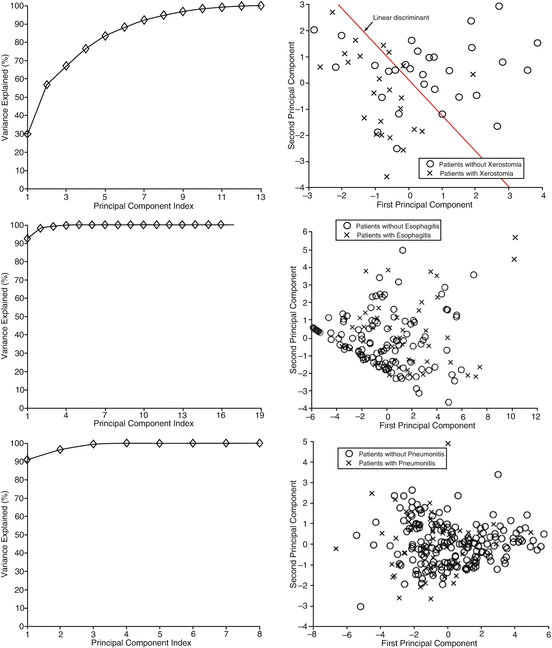
Fig. 3.1

Projection of prognostic factors for xerostomia (top), esophagitis (middle), and radiation pneumonitis (bottom) into a two-dimensional space consisting of the first and second principal components (the right column). The left column shows variation explanation versus principle component index. Linear separation in the xerostomia dataset is well demonstrated but not as much for the pneumonitis case (as seen from a wide class overlap) (Reproduced from El Naqa et al. [16])

Figure 3.1 shows three examples of PCA applied to patient data for three different prognostic challenges: prediction of xerostomia, esophagitis, and pneumonitis. The main purpose of PCA in this case is to visualize a degree of separation between patients with and without complications. For the case of xerostomia, PCA revealed several significant principal modes in the prognostic data, the first two of which accounted for only 60 % of the total varianc among the data components. However, the first two principal components already show a fairly clear distinction between the cases with and without xerostomia, meaning that the rest of the variance may not be relevant to the complication. In contrast, PCA reveals only one strong principal mode for esophagitis and pneumonitis, i.e., the original data components are so highly correlated that PCA reduces them to a single principal component. The projected data do not demonstrate clear separation among cases, which calls for a nonlinear modeling approach such as kernel methods (see Sect. 3.3.4).

3.2.2 Kernel Principal Component Analysis

Kernel PCA is a nonlinear form of the principal component analysis by use of a kernel technique (see the upcoming section on support vector machine). It is useful for detecting nonlinear behaviors in data that cannot be represented in terms of linear combination of the existing variables. The kernel trick effectively transforms an input space into a higher-dimensional feature space in which nonlinear patterns can be discoverable in a linear fashion (Fig. 3.2). However, the input space transformation does not need to be defined explicitly, as the PCA only requires the knowledge of a covariance matrix in the transformed space. The (i,j)-th component of a covariance matrix for the data x ₁, x ₂,…, x _ncan be computed directly from the kernel function $k\left(\cdot, \cdot \right)$ :

${K}_{ij}=\left\langle \varPhi \left({x}_i\right),\varPhi \left({x}_j\right)\right\rangle =k\left({x}_i,{x}_j\right)$

(3.2)

where Φ(x) denotes the input space transformation. K is then diagonalized to extract a set of principal components and corresponding eigenvalues. Kernel PCA becomes more computationally expensive than linear PCA when the number of samples exceeds input dimension. Nevertheless, when applied to problems containing nonlinear patterns (e.g., handwriting), a nonlinear PCA could be more suitable than the linear one for reducing data dimension prior to a classification task [42].

Fig. 3.2

A cartoon describing the utility of kernel PCA in linearizing a nonlinear pattern by feature transformation Φ via a polynomial kernel. The dotted lines are contour lines of the same value of projection to the first principal component (Reproduced from Scholkopf et al. [42])

3.2.3 Clustering

Cluster analysis refers to detection of collective patterns in data based on similarity criteria. It can be performed either in a supervised or unsupervised fashion. Grouping data points into clusters is useful in several ways. First, it can provide intuitive and succinct representation of the nature of data prior to major investigation. Secondly, clustering can be applied to compressing complex data distribution into a group of vectors corresponding to cluster centroids (vector quantization).

The K-means clustering is one of the most popular clustering methods. It begins with randomized partitions with the given number (K) of clusters. The partitions are then iteratively refined by the following steps: (1) an assignment step (reassignment of the cluster membership of each data point based on a distance to cluster centroids) and (2) an update step (recalculation of cluster centroids as a geometric mean of the updated membership). The Minkowski distance between the d-dimensional vectors a and b, also known as a L _pnorm, is used as a measure of proximity:

${L}_k\left(a,b\right)=\left({\displaystyle \sum}_{i=1}^d\left|{a}_i-{b}_i\right|{}^k\right)$

(3.3)

The widely used Euclidean and Manhattan distance refer to the Minkowski distance at p = 2 and p = 1, respectively.

The K-means gained popularity thanks to its simplicity and fast convergence [25]. One of the drawbacks of this algorithm is its tendency to converge to local minima when initial partitions are not carefully chosen [25]. This can be partially overcome by introducing seeding heuristis such as the K++ means algorithm by Arthur and Vassilvitskii [1]. Furthermore, the original K-means requires the number of clusters (K) to be given a priori. The choice can either be made based on domain knowledge or optimized in data in a cross-validated fashion. The optimization method employs for an objective function the Bayesian information criteria (BIC) [38] or the minimum description length (MDL) [2] that penalizes the larger number of clusters.

Another clustering algorithm gaining popularity is a neural network-derived method called a self-organizing map (SOM) or a Kohonen map [30]. In a SOM, distinct patterns in input data are represented by nodes which are typically arranged in a two-dimensional hexagonal or rectangular grid for better visualization. Each node is assigned with its location in the grid and a vector of weights on input variables. The learning algorithm begins with randomizing node weights. Then, one training example is sampled from the training set and the node at the closest distance from it (Minkowski metrics can be used) is identified as a best matching unit (BMU). The weight vectors for the BMU and the nodes in its vicinity are adjusted to decrease the distance to the training example according to the following update formula:

${w}_v\left(t+1\right)={w}_v(t)+a(t)\varLambda \left(\left|{w}_{BMU}(t)-{w}_v(t)\right|\right)\left({x}_i-{w}_v(t)\right)$

(3.4)

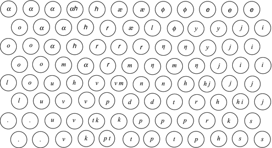
where w _v(t) is a weight vector for a node v at iteration t and x _iis the i-th input sample. The magnitude of the update is determined by the factors that depend on the distance from the BMU $\left|{w}_{BMU}(t)-{w}_v(t)\right|$ and the number of iteration (t). A window function (Λ) is the highest when $v=\mathrm{B}\mathrm{M}\mathrm{U}$ and tapers off to zero as a node goes farther away from the BMU. It ensures the nodes will be topologically ordered (neighboring nodes have similar weight patterns). The learning rate, α(t), typically decreases with iterations to ensure convergence. After the learning is repeated through all the training samples, the nodes tend to clump toward the weights that appears in input patterns frequently (topological ordering). A SOM has been shown useful in some areas such as speech recognition, linguistics, and robot control (Fig. 3.3).

Fig. 3.3

Self-organizing map learned from natural Finnish speech analysis by Kohonen [30]. Each node represents one acoustic unit of speech called a phoneme

Many challenges in bioinformatics are framed as a clustering problem, such as identifying a group of genes showing similar patterns of expression under certain conditions or diseases. A work by Svensson et al. [48] is a good example from radiotherapy toxicity modeling. They grouped 1,182 candidate late toxicity marker genes into two groups using their expression patterns in lymphocytes after radiation, although the grouping did not correlate with toxicity status. In contrast, a SOM of radiation pneumonitis risk factors built by Chen et al. [8] showed that grouping patterns among the factors can be exploited for predicting the toxicity with decent accuracy (AUC = 0.73).

3.3 Supervised Learning

3.3.1 Logistic Regression

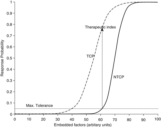
In radiation outcomes modeling, the response will usually follow an S-shaped curve. This suggests that models with sigmoidal shape are more appropriate to use [3–5, 21, 23, 24, 34, 49]. A commonly used sigmoidal form is the logistic model, which also has nice numerical stability properties. The logistic model is given by [22, 51]:

$f\left({x}_j\right)=\frac{e^{g\left({x}_j\right)}}{1+{e}^{g\left({x}_j\right)}},\kern0.46em i=1,2,\dots, n$

(3.5)

where n is the number of cases (patients) and x is a vector of the input variable values used to predict f(x _i) for the outcome y _iof the i _thpatient. The $f\left(\cdot \right)$ is referred to as the logic transformation. The “x-axis” summation g(x _i) is given by:

$g\left({x}_i\right)={b}_0+{\displaystyle \sum}_{j=1}^S{b}_j{x}_{ij},\kern0.46em i=1,\dots, n,\kern0.46em j=1,\dots, s$

(3.6)

where s is the number of model variables and the β’s are the set of model coefficients that are determined by maximizing the probability that the data gave rise to the observations (i.e., the likelihood function). Many commercially available software packages, such as SAS, SPSS, and Stata, provide estimates of the logistic regression model coefficients and their statistical significance. The results of this type of approach are not expressed in closed form as above, but instead, the model parameters are chosen in a stepwise fashion to define the abscissa of a regression model as shown in Fig. 3.4 However, it is the analyst’s responsibility to test for interaction effects on the estimated response, which can potentially be corrected by adding cross terms to Eq. 3.6. However, this transformation suffers from limited learning capacity. In such a model, it is the user’s responsibility to determine whether interaction terms or higher order terms should be added. A solution to ameliorate this problem is offered by applying artificial intelligence methods.

Fig. 3.4

Sigmoidally shaped response curves (for tumor control probability of normal tissue complication probability) are constructed as a function of a linear weighting of various factors, for a given dose distribution, which may include multiple dose-volume metrics as well as clinical factors. The units of the x-axis may be thought of as equivalent dose units (Reproduced from El Naqa et al. [14])

3.3.2 Feed-Forward Neural Networks (FFNN)

Neural networks are described as adaptive massively parallel-distributed computational models that consist of many nonlinear elements arranged in patterns similar to a simplistic biological neuron network. A typical neural network architecture is shown in Fig. 3.5.

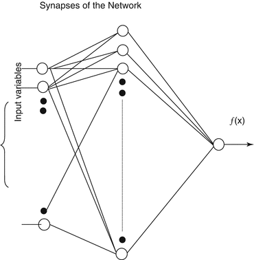
Fig. 3.5

Neural network architecture consisting of an input layer, middle (hidden) layer(s), and an output layer. The synapses of the network consist of neurons that fire depending on their chosen activation functions

Neural networks have been applied successfully to model many different types of complicated nonlinear processes, including many pattern recognition problems [41]. A three-layer FFNN network would have the following model for the approximated functional:

$f(x)={y}^T{w}^{(2)}+{b}^{(2)}$

(3.7)

where v is a vector, the elements of which are the output of the hidden neurons, i.e.,

$v=s\left({x}^T{w}_i^{(1)}+{b}^{(1)}\right)$

(3.8)

where x is the input vector and w ^(j) and b ^(j) are the interconnect weight vector and the bias of layer j, respectively, j = 1,2. In the FFNN, the activation function $s\left(\cdot \right)$ is usually a sigmoid, but radial basis functions were also used [46]. The FFNN could be trained in two ways: batch mode or sequential mode. In the batch mode, all the training examples are used at once; in sequential mode, the training examples are presented on a pattern basis, in the order that is randomized from one epoch (cycle) to another. The number of neurons is a user-defined parameter that determines the complexity of the network; the larger the number of neurons, the more complex the network would be. The number is determined during the training phase.

3.3.3 General Regression Neural Networks (GRNN)

The GRNN [44] is a probabilistic regression model based on neural network architecture. It is characterized as non-parametric, which means that it does not require any pre-determined functional form (e.g., polynomials). Instead, it estimates the joint density of input variables x and a target y from training data. The regression output using the GRNN is obtained by taking the expectation value of y for a given observation X and the joint density g(x, y):

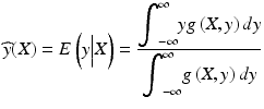
$\widehat{y}(X)=E\left(y\Big|X\right)=\frac{{\displaystyle {\int}_{-\infty}^{\infty } yg\left(X,y\right) dy}}{{\displaystyle {\int}_{-\infty}^{\infty }g\left(X,y\right) dy}}$

(3.9)

The joint density g(x, y) is estimated from training examples X _iand y _ivia the Parzen estimator where the density is regarded as the superposition of Gaussian kernels centered at the observation points with a spread σ. The resulting form of the regression function is:

$\widehat{y}(X)=\frac{{\displaystyle \sum}_{i=1}^n{y}_i \exp \left(\frac{-{D}_i^2}{2{s}^2}\right)}{{\displaystyle \sum}_{i=1}^n \exp \left(\frac{-{D}_i^2}{2{s}^2}\right)}$

(3.10)

where ${D}_i^2={\left(X-{X}_i\right)}^{\mathrm{T}}\left(X-{X}_i\right)$ , denoting the Euclidean distance between the testing data X and the i-th training data X _i.

The GRNN is fairly simple to train, with only the Gaussian width σ to be tuned. Thus, implementation of the GRNN does not require an optimization solver to obtain the weights, as in the case of FFNN. However, the output is obtained as a weighted sum of all the training samples, which could make it less efficient during running time. This could be improved by performing cluster analysis on training data (see Sect. 3.2.3) to compress it into a few cluster centers so that the metric D _ican be computed only between those center points and a testing example. The computational speed can also benefit from parallelized neural network implementation since each summation can be performed independently using synapses and an exponential activation function. In our previous work, we demonstrated that GRNN can outperform traditional FFNN in radiotherapy outcomes prediction [15].

3.3.4 Kernel-Based Methods

Kernel-based methods and its most prominent member, support vector machines (SVMs), are universal constructive learning procedures based on the statistical learning theory [50]. For discrimination between patients who are at low risk versus patients who are at high risk of radiation therapy, the main idea of the kernel-based technique would be to separate these two classes with hyper-planes that maximizes the margin between them in the nonlinear feature space defined by implicit kernel mapping. The optimization problem is formulated as minimizing the following cost function:

$L\left(x,\ \xi \right)=\frac{1}{2}{w}^Tw+C{\displaystyle \sum}_{i=1}^n{\xi}_i$