Intensity-Modulated Radiation Therapy
Arthur L. Boyer
Gary A. Ezzell
Cedric X. Yu
Introduction
The treatment techniques that are collectively known as intensity-modulated radiation therapy (IMRT) compose a broad class in a historical sequence of technical developments for improving local control of cancer by improving the physical delivery of external beam radiation. The mathematically precise geometric information about the patient’s anatomy provided by computed tomography (CT) technology enables shaping radiation fields to conform to the projection of the treatment target volume for a radiotherapy beam directed toward a tumor. General deployment of this strategy enabled shaping internally uniform fields with computer-controlled multi-leaf collimators (MLCs) (1,2,3,4,5,6,7). This class of external beam treatment techniques has been conventionally known as three-dimensional conformal radiation therapy (3-DCRT). The more beams used, the more conformal the cumulative dose in the target. A special variant of this class is the conformal arc therapy method proposed by Takahashi (8). Takahashi envisioned using an MLC to produce a continuous, smoothly connected sequence of aperture shapes that conform to the projection of the target at each gantry angle as a cone beam is continuously rotated around the patient.
3-DCRT reduces the volume of tissue that is irradiated to the prescribed dose outside the target volume, allowing higher prescribed doses to be delivered within the tumor target volume for a given level of normal tissue complications. The magnitude of the normal tissue sparing can be estimated by comparing irradiation of a spherical target volume of diameter D by either four-square, orthogonal fields that enclose the target in a cubic high-dose region of volume D3 or by many circular-shaped fields from all directions in three dimensions, ideally enclosing the target in a spherical high-dose region having a volume (4/3) π (D/2)3 = (π/6) × D3. The ratio of these two volumes of tissue irradiated to the prescribed dose is a factor of π/6 = 0.52. The clinical gain of 3-DCRT is the reduction of tissue irradiated to the prescribed dose by up to a factor of about 2. The full radiobiological advantages of 3-DCRT are a subject of research. Having less damaged normal tissue, especially vasculature, in closer proximity to the tissue stroma within the target volume appears to impart tolerance to higher prescribed tumor doses. However, for more complex tumor shapes, such as target volumes that contain invaginations, internal hollows, and bifurcations, 3-DCRT techniques using internally uniform fluence cannot deliver a complex conforming dose structure. However, one can compute modulations of the internal intensities of shaped fields (9,10,11) whose sum will produce a relatively uniform dose within a complex target shape while maintaining reduction of dose outside the target in a neighboring organ at risk. One starts with the desired result (a uniform conformal target dose that excludes organs at risk) and works backward toward incident beam intensities, earning the technique the popular name, inverse treatment planning. The beam intensities required to deliver the required nonuniform beam intensities can be produced using motion of the MLCs during the irradiation to spatially modulate the intensity, hence the name intensity-modulated radiation therapy. This chapter discusses a number of implementations of IMRT that have been put into practice.
Development of IMRT
The development of IMRT was born from the wide adoption of 3DCRT in the 1980s. Brahme et al. demonstrated (9,10) that if the intensities of radiation can be modulated across a radiation field, then the increased freedom would afford a greater ability to shape the volume of high doses, to better conform to the target than 3DCRT. Subsequent to that work, a large number of publications emerged on the use of computer optimization techniques for radiotherapy treatment planning. In 1992, Convery and Rosenbloom derived a mathematical formula for realizing intensity modulation with the dynamic movement of a collimator jaw (11). In 1994–1995, works were published to demonstrate the feasibility of using MLCs for intensity modulation of fixed-gantry fields in either a dynamic mode (continuous movement during radiation) or static mode (alternating motion of leaves with irradiation with motionless leaves) (12,13,14,15,16,17). The first clinical implementations of the IMRT technique using dynamic MLC leaf motion was at Memorial Sloan Kettering Cancer Center in 1996 using software developed in-house (18). In 1997, IMRT was first planned using commercially available software from the NOMOS Corporation and delivered using a commercially available Varian MLC at Stanford University (19).
In 1993, another form of IMRT using rotational fan beams, called tomotherapy, was proposed by Mackie et al. (20). The idea was quickly commercialized by NOMOS Corporation (21,22) with the trade name Peacock™. The NOMOS Peacock™ was the first commercial IMRT system using a dedicated short-stroke multi-vane intensity modulating collimator (MIMic), as an add-on binary collimator that opens and closes under computer control. The treatment table had to be precisely indexed from one slice to the next. For this reason, the Peacock™ device is often referred to as serial tomotherapy. Serial tomotherapy was first implemented clinically at Baylor College of Medicine in March 1994 (23). Most IMRT treatments delivered in the 1990s employed serial tomotherapy. Helical tomotherapy (HT) was then developed by Tomotherapy, Inc., as a dedicated rotational IMRT system with a slip-ring rotating gantry. It was made commercially available in 2002. More efficient delivery was achieved by continuous gantry rotation and simultaneous treatment couch translation.
In 1995, Yu proposed another form of IMRT called intensity-modulated arc therapy (IMAT) (17). Like tomotherapy, IMAT delivers photon radiation treatment over a continuous arc. Instead of using rotating fan beams as in tomotherapy, IMAT uses rotational cone beams shaped by an MLC to achieve intensity modulation. The strategy was to convert the intensity patterns into segments delivered by a sequence of arcs without table translation. Based on the fact that many beam modulation sequences can yield the same intensity pattern, it is possible to find an MLC aperture at each beam angle such that aperture shapes at successive angles are connected geometrically. The stacks of overlapping beam apertures can then be delivered with multiple overlapping arcs. An initial proof-of-principle study demonstrated that IMAT would be feasible as a treatment delivery technique. The requirement of geometric connectivity of apertures from neighboring angles adds significant complexity to the planning of IMAT treatments. IMRT is not the only way to take advantage of the geometric arrangements of the target and the surrounding avoidance structures. The CyberKnife™ system (Accuray, Sunnyvale, CA), which uses small circular x-ray beams generated by an x-band linear accelerator mounted on a robot (24) to deliver the radiation to the target, does not explicitly modulate the intensity of a beam, but is able to deliver highly conformal treatments.
The rapid adoption of IMRT shortly thereafter was facilitated by additions to the United States Federal funding mechanism for radiation oncology that occurred around the year 2000. In the late 1990s, Medicare began to introduce the hospital outpatient prospective payment system (HOPPS). As part of this system, a payment differential mechanism was included to encourage the introduction of new technology. A Medicare billing code for IMRT treatment was added to the current procedural terminology (CPT) in 2001. The technique-specific payment differential created a financial incentive to purchase treatment planning systems and linear accelerators that included cutting-edge technology for IMRT to improve quality of care, reduce health care costs, and recoup capital costs. Thus, through this explicit federal policy mechanism that encouraged “early adopters,” IMRT became available in radiotherapy centers much more rapidly than it would have otherwise (25).
IMRT has been studied extensively for the last two decades. A search on the acronym at the web sites of the major radiation oncology journals yields lists of citations numbering in the thousands. Technical issues and clinical questions are likely to be subjects of research and development for the foreseeable future.
Principles of IMRT Planning and Delivery
Up to a point, treatment planning for IMRT differs little from treatment planning for 3DCRT. The concepts introduced by the International Commission on Radiation Units and Measurements (ICRU) No. 50 are applied to delineate a planning target volume (PTV) as an expansion of a clinical target volume (CTV) that is in turn based on a gross tumor volume (GTV). The expansions are theoretically based on uncertainties in the segmentation, patient positioning, and respiration motion during treatment, and the displacement of structures by physiological processes from one treatment day to the next. An extension of digital imaging and communications in medicine (DICOM) formats, the DICOM-RT format, is the standard for file transfers of imaging studies, structure sets, dose distributions, and treatment sequences. Computer workstations are commercially available for segmenting the target structures and the normal structures using diagnostic studies. Geometric correlation of the disparate studies (CT, MRI, and PET/CT), known as fusion, allows the radiation oncologist to take advantage of the imaging advantages peculiar to each type of study. The radiation oncologist can identify the 3D surfaces of these structures by drawing contours along their boundaries in sequential reconstruction planes using a growing suite of artificial-intelligence segmentation tools.
The way IMRT, including IMAT and tomotherapy, spares critical structures is by redistributing the normal tissue dose to less critical regions and by reducing the high-dose volume to just cover the target. For a given case, the geometric arrangement of the target and its surrounding avoidance structures dictates the preferred beam angles, and along each beam angle, the preferred locations at which the radiation is delivered to the tumor. The calculation of fluence required to achieve a desired dose distribution bears certain similarities to the reconstruction of CT scans. How IMRT fluence profiles may be computed has been illustrated by Bortfeld and Webb (26) based on earlier work by Brahme (9) using a simplified two-dimensional (2D) model. This 2D test case contains an OAR of radius r0 embedded within the side of a PTV of radius r (Fig. 13.1). The OAR is centered on (x0, y0) = (0,-4). Using the approximations and methods similar to Brahme (9), an analytic ideal fluence, φ, for a continuous arc field
as a function of gantry angle φ can be calculated based on three conditions on rays passing through the PTV and OAR structures:
as a function of gantry angle φ can be calculated based on three conditions on rays passing through the PTV and OAR structures:
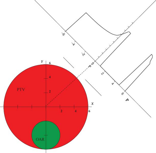 Figure 13.1. Geometry of simple two-dimensional (2D) test case. The planning target volume (PTV) consists of a circle whose radius is r = 4 cm. The OAR is a circle whose radius is r0 = 2 cm and is embedded at the bottom side of the PTV. An ideal fluence can be calculated analytically for this case. The fluence in the solution at an angle φ = 45 degrees is depicted as a function of the distance from the center of the treatment beam, p. |
where
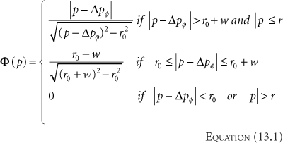
Rays that meet the first condition pass through the PTV and are modulated to compensate for rays that are excluded because they pass through the OAR. Rays that meet the second condition pass within a distance w of the OAR. Their amplitudes are cut off at the fixed value given in the equation to avoid a singularity of infinite magnitude that would otherwise exist at the boundary of the OAR. Rays that meet the third condition are set to zero because they either pass through the OAR or pass outside the PTV. A one-dimensional (1D) beam fluence calculated for an angle φ = 45 degrees at which the beam is directed toward the center of the PTV is shown in Figure 13.1. The entire computed fluence is illustrated as a sinogram plot of fluence across the beam as a function of gantry angle in Figure 13.2. This approach allows no fluence to be directed through the OAR resulting in a zero-fluence valley through the sinogram in Figure 13.2. This simple idealized inverse solution can be modified to apply to tomotherapy and fixed-gantry multiple-field IMRT by using the appropriate parts of the sinogram in Figure 13.2. A search for a generalized 3D analytic inverse solution has not as yet yielded a widely applicable and practical solution (27). The most fruitful approach has been to calculate practical fluence distributions numerically using an optimization scheme based on a cost function that reflects some quantitative assessment of the dose distribution that a calculated fluence will deliver. These schemes generally allow some fluence to pass through the OARs to build up a dose in the PTV. Over the last decade, many new methods of treatment delivery using multiple fixed beams or rotating beams have been developed. No matter what form of delivery is
used, the radiation dose is delivered to the target through multiple radiation fields of varying sizes and shapes. To take full advantage of the geometric arrangements of a specific clinical case, a large number of fields, also referred to as segments, subfields, or apertures, is needed. The number of field segments is case dependent and in general, the more complex the geometric arrangement, the larger the number of field segments required to achieve the optimal plan (28). Where these apertures are placed—within a limited number of beam angles or spaced around the patient as one or more arcs—has been shown to be less important through plan quality comparisons.
used, the radiation dose is delivered to the target through multiple radiation fields of varying sizes and shapes. To take full advantage of the geometric arrangements of a specific clinical case, a large number of fields, also referred to as segments, subfields, or apertures, is needed. The number of field segments is case dependent and in general, the more complex the geometric arrangement, the larger the number of field segments required to achieve the optimal plan (28). Where these apertures are placed—within a limited number of beam angles or spaced around the patient as one or more arcs—has been shown to be less important through plan quality comparisons.
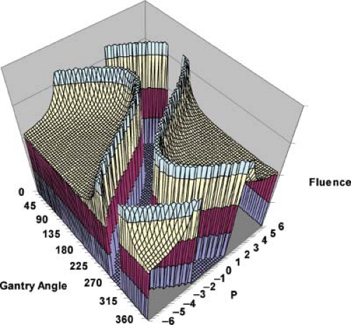 Figure 13.2. The computed fluence (arbitrary units) as a sinogram plot of fluence across the beam as a function of gantry angle. This calculation required that no fluence be delivered to the OAR resulting in the region of zero fluence that winds across the sinogram. |
 Figure 13.3. A depiction of a beam viewed as a bundle of beamlets. Each beamlet in the bundle can be identified by a row index, l and a column index, m. The fluence within each beamlet is proportional to the beamlet weight or bixel value, wl,m. |
Rotational deliveries generally spread the normal tissue dose to a greater volume of normal structures than IMRT methods employing a limited number of fixed gantry beam directions. The key principle is that to deposit a given integral dose to the target, it is necessary to deposit an irreducible integral dose to the surrounding structures (a transit dose), as dictated by the physics of dose deposition. IMRT is appropriate for clinical cases in which delivering a lower dose to a larger volume of normal tissue is better than delivering a larger dose to a smaller volume of normal tissue. Accordingly, volume considerations must be carefully given for parallel organs, such as the lung, and for pediatric applications.
The dose prescription for IMRT is more structured and complex than the single-valued prescription used to guide pre-IMRT therapy. Ideally, one would prescribe some dose value to every voxel in the patient. In practice, blocks of high therapeutic dose and dose limits are prescribed to fractions of the target volume containing many voxels, and dose limits are assigned to fractions of the OAR. A dose calculation is built up within a calculation matrix using some form of x-ray beam modeling. The dose calculation is based on the beamlets associated with each treatment beam (Fig. 13.3). For a beam directed toward the patient from a given angle, the elements of the 2D array of beamlet weights, wl,m (arranged in rows labeled with an index l, and columns labeled with an index m) are termed bixel weights. The beam intensity map will be proportional to the matrix of bixel weights. A set of bixels, wk,l,m, is associated with the k beam direction (Fig. 13.4). This 3D set of
beamlet weights drives the dose calculation in the 3D voxel matrix, Dc(x, y, z) = Dc(r). The dose calculation that estimates the dose delivered by each beam is based on the values in the beam’s bixel matrix. Once the dose is calculated for every beam, the voxels within the patient’s skin surface will contain the calculated dose values. The goal of the optimization process is to select those bixel weights that deliver the most favorable dose distribution. The dose distribution is assessed using some mathematical technique for approximating the subjective medical value of the shape and magnitude of the computed dose distribution. This assessment is called the cost function, or alternatively, the objective function. The simplest cost function simply computes the square of the differences between the computed dose, Dc(r), and doses prescribed for the target volumes and the OARs, Dp(r).
beamlet weights drives the dose calculation in the 3D voxel matrix, Dc(x, y, z) = Dc(r). The dose calculation that estimates the dose delivered by each beam is based on the values in the beam’s bixel matrix. Once the dose is calculated for every beam, the voxels within the patient’s skin surface will contain the calculated dose values. The goal of the optimization process is to select those bixel weights that deliver the most favorable dose distribution. The dose distribution is assessed using some mathematical technique for approximating the subjective medical value of the shape and magnitude of the computed dose distribution. This assessment is called the cost function, or alternatively, the objective function. The simplest cost function simply computes the square of the differences between the computed dose, Dc(r), and doses prescribed for the target volumes and the OARs, Dp(r).
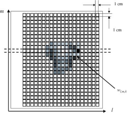 Figure 13.4. An example of a beam intensity map. Each square represents a bixel. The rows are labeled with an index l. The columns are labeled with an index m. This intensity map is associated with a beam direction determined by gantry angle and couch rotation labeled with an index k. Each square represents a bixel with a weight wl,m,k. The bixels in which the beam is always blocked by MLC leaves are displayed as white. Shades of gray are used in this figure to indicate levels of beam intensity, wl,m,k, black corresponding to the highest intensity. |
where i is the structure index and Ci is the weighting factor used to stress the relative importance of different structures. As the computed dose distribution becomes more similar to the prescribed dose distribution, the value of this cost function decreases. Therefore, the goal of the optimization procedure is to minimize F. What is not shown explicitly in Equation 13.2 is the assignment of dose prescriptions to the planning structures; the target volumes and the OAR. The quadratic cost function given in Equation 13.2 also does not differentiate the target and the OARs. In realistic cost functions, lower doses in the OARs than the prescribed dose limit will be encouraged rather than penalized. Many other measures of the “goodness” of the computed treatment plan have been investigated. Particularly, intriguing are cost functions based on nonlinear tumor response models. Another very general approach is to create a cost function that is itself a summation of many “costlet,” functions of relevant parameters such as dose points on the dose–volume histograms (DVH), tissue complication probability, normal tissue complication probability, equivalent uniform dose, and so on. A dose–volume minimum objective is usually applied to a target structure. This objective is met if the dose calculated in all voxels that make up a specified percent of the designated structure volume is greater than or equal to the structure dose objective value.
IMRT is most commonly delivered using the MLC. There are two basic ways to use the MLC (29). One method, called the step-and-shoot or segmented multileaf collimation (SMLC) approach, alternates between setting MLC apertures without delivering dose and delivering small increments of dose without moving the MLC leaves (30). The dose delivered by SMLC along a beamlet is determined by the amount of time the beamlet remains in an open gap between opposed MLC leaves. The other method, called the sliding window or dynamic multileaf collimation (DMLC) approach, employs an MLC control system that can deliver dose while simultaneously moving the leaves by interpolating leaf positions between control points (15). The dose delivered by DMLC along a beamlet is determined by the amount of time the beamlet remains in the gap between continuously moving opposed leaves. There is little, if any, intrinsic difference between the two methods if they are implemented with equivalent fast computer-controlled electromechanical systems.
In both serial and HT implementations, intensity modulation is achieved with a binary MLC, consisting of two opposing banks of tungsten leaves operating in either open or closed states. When all the leaves are open, the binary MLC shapes a fan beam with a width equal to the total leaf travel of the two opposing leaves. Each of the two rows of beamlets is independently controlled to open and close by a computer, and the fraction of time a beamlet is open determines the relative intensity of the beamlet. As this fan beam continuously rotates around the patient, the relative intensities of the beamlets are adjusted with the opening and closing of the corresponding leaf of the binary collimator, allowing the radiation to be delivered to the tumor through the most preferable directions and locations of the patient.
Both serial and HT systems offer a “turn-key” approach to IMRT implementation with the planning system specifically designed for the delivery unit. The Peacock™ system, developed by NOMOS Corporation, optimizes beam intensities for a sequence of 55 radiation beams (every 5 degrees) around the patient based on dose constraints using a simulated annealing optimization algorithm. It encompasses most of the features of current inverse treatment planning systems as described by Carol et al. (22,23). Because the serial tomotherapy uses an add-on device to an existing linac, non-coplanar arcs with the couch at a small angle to its default position are also allowed. HT utilizes a dedicated ring gantry and a computer-controlled couch. The treatment plan is delivered through a 6 MV x-ray fan beam in continuous rotation around the long axis of the patient while the patient is slowly translating through the gantry aperture at a constant speed, which is predetermined by the pitch factor and the gantry period. Each gantry rotation is approximated by 51 equally spaced static beam projections with 64 binary MLC leaves in each projection. Both serial and HT achieve intensity variations of the beamlets with a binary MLC. The degree of modulation by the binary MLC is determined by the gantry period, the modulation factor, and the inherent transit time of leaf motion (<40 ms). Because each MLC is individually controlled and allows full intensity modulation at each projection during dynamic gantry rotation, the degree of intensity modulated is less constrained as compared to MLCs that move continuously to shape extended radiation fields. Therefore, theoretically speaking, tomotherapy provides a planning system with greater freedom to use highly modulated beams than MLC delivery of IMRT employing fixed cone beams.
When a broad photon beam is collimated into a fan beam with the width of only that of two beamlets, most of
the x-ray photons generated in the target are blocked, leading to inefficient usage of the monitor units (MUs) and long treatment times for large targets. To compensate for the inefficiency, HT uses a high dose rate of 880 MU/min. The gantry rotation period ranges from 15 to 60 seconds, depending on the fractionation size, the modulation factor, and the pitch. The width of the fan beam can also be preselected in a range of 1.0 to 5.0 cm as a trade-off between the resolution of the intensity pattern and the delivery efficiency.
the x-ray photons generated in the target are blocked, leading to inefficient usage of the monitor units (MUs) and long treatment times for large targets. To compensate for the inefficiency, HT uses a high dose rate of 880 MU/min. The gantry rotation period ranges from 15 to 60 seconds, depending on the fractionation size, the modulation factor, and the pitch. The width of the fan beam can also be preselected in a range of 1.0 to 5.0 cm as a trade-off between the resolution of the intensity pattern and the delivery efficiency.
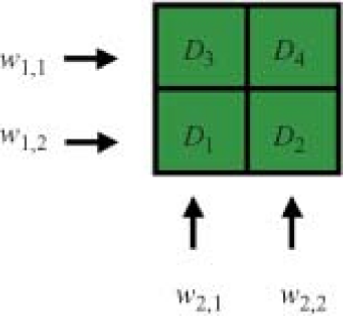 Figure 13.5. A simplified dose calculation matrix used to illustrate inverse treatment planning optimization. In order to make the example easy to calculate, a two-dimensional (2D) matrix consisting of only four voxels is considered. Voxels 1, 3, and 4 are the target structure and voxel 2 is an avoidance structure. In the example shown here, the prescribed dose values (in arbitrary units) in the voxels are set to D1 = 1.0, D2 = 0.5, D3 = 1.0, and D4 = 1.0. Two simplified beams are shown schematically. The bixels in a lateral beam have initial weights w1,1 and w1,2. The bixels in the vertical beam are indicated to have weights w2,1 and w2,2. The objective of the optimization is to select weights for the bixels that cause calculated doses in the voxels to be as close as possible to the prescribed doses. For this example, the initial bixel values for Beam 1 will both be set to 0.5 and the initial bixel values for Beam 2 will be set to 0.4. |
Treatment Planning for IMRT
The cost function, F(wi), can be considered to be a function of a space whose dimension is the number of variables, that is, the number of beamlet weights. For IMRT, this is something on the order of 10,000 variables depending on the size of the beamlets, the size of the fields, and the number of beams. A sophisticated computer algorithm is required to minimize the cost function efficiently and effectively. A number of such algorithms have been implemented and are available commercially. To gain an appreciation of how this optimization process works, we will consider a very simple case using a 2D dose matrix containing only four voxels labeled (1) to (4) in Figure 13.5. Three of the voxels, (1) to (3), contain a target for which the dose prescription Dp = 1 and one voxel (4) contains an organ at risk for which the prescription will be Dp = 0.5. The dose is to be delivered by two beams, one directed horizontally and one delivered vertically. Each beam contains only two beamlets. For example, beamlet 1 of beam 1 irradiates voxels 1 and 2, and beamlet 2 of beam 1 irradiates voxels 3 and 4. A flow diagram of an iterative procedure for optimizing the bixel values is illustrated in Figure 13.6. One starts with an initial guess at the beamlet weights. One calculates the doses delivered by these weights and then compares the dose computed in the voxels with the dose prescribed for the voxels by a const function. Many different cost functions have been employed experimentally and commercially. One cost function computes the average dose difference along the beamlet path through the dose matrix. If the dose averaged over the beamlet voxel path is too large, one reduces the beamlet weight. If the dose in the voxels is too small, one increases the beamlet weight. To carry out this step, one needs a table that maps the beamlets to the voxels and vice versa. One then continues to the next beamlet until all the beamlets have been adjusted for all the voxels. At this point one has computed an entirely new set of beamlet weights. Next, one recomputes the dose distribution with this revised set of beamlet weights (as in Fig. 13.7). Then, one starts at the first beamlet again, and makes adjustments throughout a second iteration. By repeating this cycle many times, one gradually approaches a stable set of beamlet weights (Fig. 13.8). The cost function is used to assess the progress of the
algorithm. For this example, the cost function is given in Figure 13.9. In this example, after 10 iterations, the cost function no longer changes significantly with further iterations. At this point the algorithm has done about as well as it can do. For this example, the dose matrix after 10 iterations is given on the right side of Figure 13.7. The prescribed doses were not achieved. However, the achieved dose is within ∼10% of the prescribed dose and a clinically significant difference was achieved between the dose to the target volume and the dose to the organ at risk. The dose to the target volume was not uniform. However, it is uniform within a tolerable range. Similar features are generally exhibited with the inverse planning for clinical cases for which the numbers of voxels, bixels, and beams are considerably greater than this illustrative calculation.
algorithm. For this example, the cost function is given in Figure 13.9. In this example, after 10 iterations, the cost function no longer changes significantly with further iterations. At this point the algorithm has done about as well as it can do. For this example, the dose matrix after 10 iterations is given on the right side of Figure 13.7. The prescribed doses were not achieved. However, the achieved dose is within ∼10% of the prescribed dose and a clinically significant difference was achieved between the dose to the target volume and the dose to the organ at risk. The dose to the target volume was not uniform. However, it is uniform within a tolerable range. Similar features are generally exhibited with the inverse planning for clinical cases for which the numbers of voxels, bixels, and beams are considerably greater than this illustrative calculation.
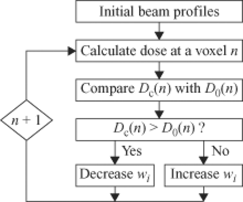 Figure 13.6. A Schematic flow diagram of an iterative process for optimizing the simple example. |
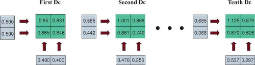 Figure 13.7. The doses computed using bixel values at the first, second, and tenth iteration steps in the simple example. |
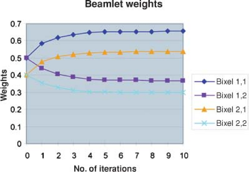 Figure 13.8. Plot of bixel values for beamlets in the simple example as a function of iteration number. After about the fifth iteration, the beamlet weights have converged. |
Different algorithms use different search strategies to minimize the cost function. One search strategy changes beamlet weights along the descending gradient of the cost function, F(wi). One selects an initial set of beamlet weights, wi = (w1, w2, w3, …), the cost function F(wi), and the local down-hill gradient, –grad F(wi). On selects a step size Δi to compute weights that take a step from wi to the point wi + Δi along the down-hill direction of the gradient. After taking this step, one recomputes the dose distribution based on the revised beamlet weights along with a revised value of the cost function and repeats the process. This method will find the minima in the cost function F(wi) nearest to the starting point. This process is conceptualized in Figure 13.10, a cost function for the simple illustrative case. In this case, the cost function space has four dimensions, but only two dimensions associated with the two beamlet weights of beam 1 are given in Figure 13.10. The minimum found by the iterative procedure is illustrated. Unfortunately, there is no guarantee that there is only one minimum in every case. If the optimization algorithm gets trapped in a local minimum far from the global minimum, the treatment plan may be unsatisfactory. Nevertheless, variants of the down-hill gradient search approach are used widely in commercially available treatment planning systems.
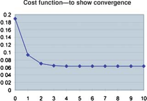 Figure 13.9. Plot of the cost function used for the simple example as a function of iteration number. The cost function has reached a stable value of about 0.06 after 10 iterations, close to an asymptotic limit. |
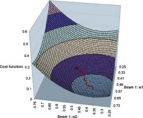 Figure 13.10. A graph of the cost function surface computed in two of the four dimensions of the bixel space for the simple example. The bixel values for Beam 2 were fixed at their optimal values, and the portion of the cost function surface was computed as a function of a range of bixel values for Beam 1 in the vicinity of their optimal values. The locus of the starting values used in the iteration for the bixels of Beam 1 (0.5) is indicated by a small oval. The trajectory of the iterative process is indicated schematically by a red path. The optimal bixel values (w1,1 = 0.655 and w1,2 = 0.368) are found at the minimum of the cost function surface where the cost function is slightly over 0.06 in this example. |
To avoid getting trapped in a local minimum, simulated annealing uses a stochastic strategy, whereby some uphill changes are accepted in addition to the down-hill changes (Fig. 13.11). As long as a change ΔF in the cost function F is negative (e.g., the plan is being improved), the change in a beamlet weight is accepted. When the change in the beamlet weight results in an increase in the cost function, a probability of accepting the change is computed using P = exp(-ΔF/kT) where kT is a variable that is used to gradually decrease the probability of accepting an uphill change as long as the search continues. This allows the
search to get out of local minima into deeper minima that may be nearby as illustrated schematically in Figure 13.11.
search to get out of local minima into deeper minima that may be nearby as illustrated schematically in Figure 13.11.
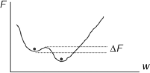 Figure 13.11. A schematic plot illustrating a cost function as a function of a generalized bixel vector, w. The cost function is shown to have two minima. By using simulating annealing, the search for the minimum is given a chance to escape from the higher minimum and enter into the lower minimum. |
Intensity Modulation
It is fairly obvious that the shape of a 1D beam profile delivered by a static or dynamic leaf sequence is determined by the positions of the leaf ends set at each instance or control point of the sequence. It is also easy to see that there is more than one way to achieve a given profile. This is illustrated in Figure 13.12. The top of the figure depicts a simple 1D ideal fluence pattern having a maximum of three levels near one end. Any completely described profile of finite length must, by definition, start and end at zero intensity. To reach a single maximum of M levels, the profile intensity must increase by M fluence steps (delivered as some fixed number of MUs in each step). Each step up is counted as a setting of a leaf whether the leaf moves or not (assume that it is the left-hand leaf in Figure 13.12, designated the A-leaf). After reaching the maxima, the profile intensity must be decreased by M steps down at positions where the right-hand leaf (designated the B-leaf) has been positioned. The six sequences depicted in the lower portion of Figure 13.12, each consisting of three instances, all sum up to the profile in the top of the figure. It has been pointed out that any SMLC profile with a single maximum that requires M leaf-end positions could be created by M! unique sequences (31). In Figure 13.12, the first sequence is a “close-in” strategy that starts with the largest extent of the profile and closes down on the maxima. The last instance depicted in Figure 13.12 is the sweeping window strategy that will be described in the subsequent text. In the case illustrated in Figure 13.12 there are M! = 3! = 6 unique sequences. The order in which the leaves are set in these sequences is not considered in this calculation. If you consider all permutations of the instances in which the positions are set, there are (M!) (2) possible sequences.
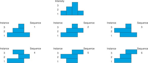 Figure 13.12. Six different sequences that all create the same intensity profile. The top center subfigure is the profile, intensity plotted against positions across the field. The bottom six subfigures show different sequences of three gaps that all lead to the same cumulative intensity profile. |
Intuitively, as the profile becomes more structured, the number of possible sequences will increase. Webb considered the more general case in which there are multiple maxima (32). The calculation is illustrated in Figure 13.13. A 1D profile is shown with peak intensities of levels H1 and H2. In general, there can be multiple maxima with levels H1, H2, H3, …, each peak characterized by a change in gradient of the profile from positive to negative. In general, let max be the total number of maxima. Between any two maxima is a minimum that drops to P1, P2, …, each minimum is characterized by a change in slope of the profile from negative to positive. The two potential minima at the beginning and end of the profile are not counted. Therefore, there will be max – 1 such minima. Webb (32) has shown that the number of physically achievable leaf sequences that produce the discrete profile is given by
This can be a very large number of possible step-and-shoot types of sequences that all create the same discrete
profile. However, for the 1D case, one can still carry out an exhaustive search for a solution that is, in some sense, optimal. For MLC systems that do not allow inter-digitations and leaf-end abutment, the number of physically achievable sequences is smaller. The reduction depends on the details of the MLC system. Webb has calculated a typical value for an Elekta MLC to be ≈1094. In general, an exhaustive search of all possible 2D leaf sequences for an optimal leaf sequence is impractical. Either the delivery sequences must be computed by some specific algorithm or an efficient optimization algorithm must be used to search iteratively for an optimum in this large search space.
profile. However, for the 1D case, one can still carry out an exhaustive search for a solution that is, in some sense, optimal. For MLC systems that do not allow inter-digitations and leaf-end abutment, the number of physically achievable sequences is smaller. The reduction depends on the details of the MLC system. Webb has calculated a typical value for an Elekta MLC to be ≈1094. In general, an exhaustive search of all possible 2D leaf sequences for an optimal leaf sequence is impractical. Either the delivery sequences must be computed by some specific algorithm or an efficient optimization algorithm must be used to search iteratively for an optimum in this large search space.
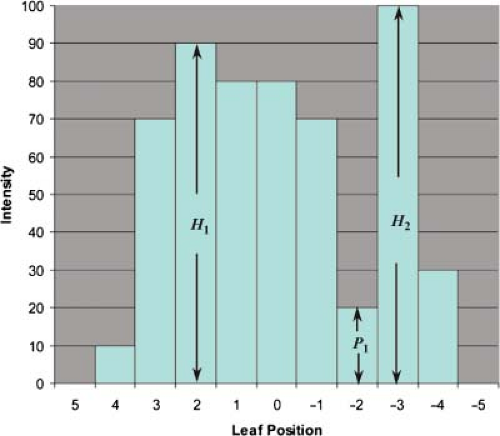 Figure 13.13. A more general one-dimensional (1D) beam profile that contains two maxima separated by a single minima. The total number of different sequences that can produce this profile is 9! X 10!/2! = 6.58 × 10¹¹. |
Given that one has at hand the technical means to create DMLC and SMLC leaf sequences, and given that there are multiple sequences (in fact, billions) possible for richly structured intensity-modulated beams, what is the best way to determine a leaf sequence to deliver a desired intensity-modulated beam? Methods by which arbitrary x-ray beam intensity profiles may be produced through dynamic jaws or MLCs have been extensively investigated (11,12,15,16,33,34,35,36) considering exhaustive searches, optimization iteration, linear programming, or direct aperture computation to minimize the total beam delivery time.
One commonly used dynamic delivery technique is the so-called sliding window or DMLC technique where both leaves start at one side of the area to be irradiated and move unidirectionally, at different speeds, to the other side (15). The intensity profile to be delivered consists of linear segments of straight lines between closely spaced control points. The delivery is realized by a series of velocity-modulated motions of the leaves with the x-ray beam delivering dose at a constant dose rate.
The required intensity pattern can be expressed as Φj(xi) = MUi,j where i (an index locating a point along a leaf trajectory) and j (an index numbering leaves) are indices for the 2D coordinates of finite pencil beams. The leaf sequence trajectory consists of specifications of the positions of the two leaves in each opposing leaf pair as a function of accumulated MUs during the delivery of the field. We will use the convention that the leaves move from left to right and that leaf A will be the trailing leaf on the left and leaf B will be the leading leaf on the right. The sequence of leaf positions along the X-axis can be denoted as XA(MUn) and XB(MUn), where the index n enumerates the sequence of the cumulative meter-set weight (CMW). We will plot the leaf trajectory by placing the independent variable, CMW, on the ordinate axis (Y-axis) and the dependent variables, the A-leaf and B-leaf positions, on the abscissa axis (X-axis). In the practical implementation, the trajectories are ordered pairs of numbers. In each pair, one number is the leaf position and the other is the CMW.
Let Φ(x) be the fluence down the center of the trajectory of a leaf pair. One way to deliver a prescribed fluence is to determine the arrival “times” at x, tA(x) for leaf A and tB(x) for leaf B. The units of the arrival times are expressed in units of CMW. The irradiation “time” interval at x between the opening of a beamlet by leaf B and the shielding of a beamlet by leaf A can be written as
The maximum velocity that the leaves can move is Vmax. The leaf velocity as a function of the leaf position for the dynamic leaf sequence has been derived independently by several authors:
where the positive sign applies to regions of positive fluence gradient and the negative sign applies to regions of negative fluence gradient. The leaves start the sequence closed at the left side of the field and end the sequence closed together at the right side of the field (e.g., Fig. 13.14). In the initial region and in any subsequent region in which the fluence gradient is positive, the leading leaf, B, moves with the maximum velocity and the trailing leaf A moves along a trajectory with a modulated velocity determined by the fluence profile gradient (see preceding equation). In those regions in which the fluence gradient is negative, the trailing leaf, leaf A, moves with the maximum velocity, while the leading leaf moves along a trajectory determined by the velocity as calculated in Equation 13.5. The DMLC method is a highly efficient delivery technique because the beam does not have to be switched off during the delivery process. However, the quality assurance (QA) procedures for this technique require consideration of the precise location of the effective radiation field edge and the stability
of leaf speed to ensure that the DMLC performs in accordance with the instruction of the leaf sequence file.
of leaf speed to ensure that the DMLC performs in accordance with the instruction of the leaf sequence file.
Related posts:


Stay updated, free articles. Join our Telegram channel

Full access? Get Clinical Tree


