High Dose-Rate Brachytherapy Treatment Planning
Bruce R. Thomadsen
General Considerations of High Dose-Rate Brachytherapy Treatments
High dose-rate (HDR) brachytherapy forms a special method of delivering brachytherapy where the treatment session lasts a short time. What constitutes “a short time” is considered below, but in the overview, the treatment session takes from 20 minutes to a couple of hours, as opposed to a day to several days for conventional, low dose-rate (LDR) brachytherapy. Most of treatment planning for HDR brachytherapy remains identical to that for general brachytherapy, which is covered in Chapter 8. This chapter will only consider those aspects of treatment planning that are either unique for, or of much greater importance to, HDR planning. The discussion that follows does not go in order of steps to perform for an HDR application. For example, planning a brachytherapy procedure, which constitutes the first step, comes late in the chapter. One reason for not following the procedural order is that the order varies depending on the nature of the procedure. However, the main reason is that the principles covered early in this chapter must be understood before applying them in planning.
Several methods have been used in the past to deliver the treatment in the short time, but all units currently use the same principal—a very intense radioactive source on a computer-controlled cable steps through the target volume, pausing for specified periods at particular locations along the way. The pausing locations are referred to as dwell positions, and the duration for which the source pauses are dwell times. Often, the dwell times are normalized to a particular dwell time location or the maximum, in which case the normalized values are called dwell weights. A unit that operates in such a manner is called a stepping source device. The radioactive source for most units is 192Ir, although some use 169Yb, or two sources, one each of iridium and ytterbium. Some very old units use 60Co. The operation of HDR units is discussed in detail in many texts (1,2). Since this chapter deals with the treatment-planning aspect of HDR brachytherapy, further description of the units proper is left to the reader’s initiative.
HDR brachytherapy offers several advantages over LDR brachytherapy.
Improved dose optimization capability. In an HDR brachytherapy application, the dwell positions perform the same role as the source positions do for LDR brachytherapy. For example, the same locations where individual iridium sources would fall in an LDR gynecological implant, the single HDR source would pause for a dwell position. Such an LDR implant could, and should, be “optimized.” “Optimization,” in this context, means adjusting the strength or positions of the sources to obtain a dose distribution with specified, desired characteristics (3). One optimization goal often is simply that a specified isodose surface covers a target volume. Other optimization criteria might include a specified required homogeneity for the dose through the target volume, or the maximum dose allowed to other anatomical structures. Optimization of a medium size LDR implants often requires 8 to 10 different source strengths, which sometimes becomes difficult to obtain from a supplier. For a similar HDR unit, the dwell times at each dwell position, on the other hand, commonly may vary in increments of 0.1 second from 0 to 999 seconds. Thus, satisfying the optimization requirements becomes easier with the great flexibility in relative strength at each dwell position. Optimization plays such an important part in HDR treatment planning that a section of this chapter is devoted to this topic.
More stable positioning. For intracavitary insertions, HDR applicators usually lock into their treatment positions through fixation to the treatment couch. With the patient essentially immobilized (e.g., in stirrups and strapped to the table), the applicator moves little between imaging for dosimetry calculations and the completion of the treatment session. One series studying the movement of HDR tandem and ovoid applications reported an average movement based on skeletal anatomy of 2 mm (4). This compares with an average of 2 cm movement for LDR tandem and ovoids (5).
Adding distance to normal tissue. For some HDR treatments—notably gynecological intracavitary insertions or head and neck interstitial implants—normal tissue structures can be pushed away from the path of the source during the treatment, reducing their dose. While not every treatment site can use this technique, in those for which it applies the dose reduction to normal structures can be marked. In general, the discomfort that similar tissue displacement would cause over the multiple-day treatments for LDR brachytherapy would be intolerable.
Outpatient treatment. The driving force that led to the wide use of HDR brachytherapy was the economic shift in reimbursement it produced from the inpatient hospital to the clinical facility that delivers the HDR treatments. This occurs because most HDR treatments are delivered on an outpatient basis. In addition to changing the revenue patterns, outpatient treatments usually are much more convenient and comfortable for the patients than confinement in a hospital room in radiation isolation.
Smaller applicators. For gynecological intracavitary applications, the tandem used for HDR treatment of uterine cancer has only a 3-mm diameter compared with the 7-mm diameter tandem used for LDR brachytherapy. The dilation required to insert the LDR tandem forms the most painful part of the treatment procedure. By comparison, the sound used to measure the length of the uterine cavity before dilation takes place is also 3-mm in diameter and often requires no anesthesia.
Intraoperative and perioperative treatments. For interstitial cases, HRD brachytherapy treatment can commence immediately following insertion of the applicator or catheters, localization imaging, and dose calculations. LDR brachytherapy cases usually require ordering the sources, or if sources were ordered ahead, performing the implant as planned without the possibility of modifications based on new information noted during the operative procedure. This ability to treat immediately after placement, along with the short duration of treatment, opens the possibility of using HDR brachytherapy during operative cases (intraoperative) for irradiation of tumor beds during resection or for wider use of image-guided implants (6).
Reduction of radiation exposure to health care providers. The final advantage of HDR brachytherapy is that all personnel leave the treatment room for the actual delivery of the radiation, and with adequately shielded walls and doors, the radiation exposure to staff should remain minimal.
HDR Brachytherapy also has disadvantages compared with LDR brachytherapy.
Treatment unit complexity. Compared with the usual LDR brachytherapy situation of sources manually inserted into an applicator, the HDR situation seems much more complicated. With the treatment unit, transfer tubes to guide the source between the unit and the applicator, transferring treatment programs between the treatment planning computer and the treatment unit computer, HDR brachytherapy entails a host of considerations not applicable to LDR brachytherapy.1
Compressed time frame. Adding to the complexity of HDR brachytherapy, much of the action takes place in time frames short compared with LDR brachytherapy. For example, after insertion of a tandem and ovoids for cervical cancer therapy, making images and calculating the treatment program, the actual delivery of the treatment frequently takes 10 to 30 minutes. If there were an error in the treatment program, it would be easy for the error to be executed before detection. The situation with LDR treatments provides some latitude for detecting errors. The long duration of the treatment gives more opportunity to spot and correct errors well before the end of treatment, when corrective actions could prevent serious injury.
Radiobiological disadvantage. The most serious disadvantage for HDR brachytherapy results from radiobiology. Radiobiology is also such an important aspect of HDR brachytherapy that it has its own section below. In the current discussion, it suffices to say that compared with LDR brachytherapy, radiation delivered at a HDR produces a greater increase in damage to normal tissue compared to cancerous tissue.
The potential for very high radiation doses resulting from mechanical failure. The HDR source cable can become stuck or snagged, or the source can break free from the cable. In either case, the patient could receive an injurious amount of radiation in about 1 minute. While the operator is unlikely to receive an injurious amount of radiation removing the stuck source from the patient, there is a real potential for receiving exposures in excess of allowed limits.
Radiobiological Considerations
Therapeutic Ratio
Accomplishing the goal of radiotherapy requires inflicting more damage to diseased cells than to normal tissue cells. The therapeutic ratio is an important measure involved in the planning for the goal of uncomplicated cure of disease. The therapeutic ratio could be defined as the ratio of the damage to tumor cells to that to normal cells for the same delivered dose, or
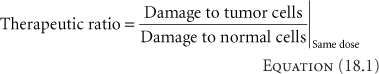
Since it becomes difficult to grade damage, and the damage to cells is not linear with dose, a more common equivalent expression often forms the basis for the calculation of this ratio, determining the ratio of the doses required for the same biological endpoint, for example, five logs of cell kill. The equation becomes
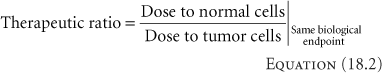
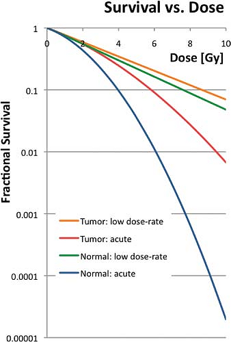 Figure 18.1. A cell survival curve, plotting the fraction of cells surviving a single exposure to radiation as a function of the dose delivered. The curves are based on α = 0.25 Gy-1, βtumor = 0.025 Gy-2, βnormal tissue = 0.083 Gy-2, μrepair = 1.5 h-1. Cell proliferation has been ignored. |
The more effective the radiation is at killing a certain type of cell, the lower the dose required to reduce a population of cells to a given level.
Figure 18.1 shows a typical curve relating the survival of cells to dose of radiation. In general, the relationship between cell survival, S, and cell killing can be modeled as
where D indicates the dose delivered. Equation 18.3 is just a model, and should not be taken as the true description of the physical and biological process. In the figure, the lines labeled “Normal Acute” and “Tumor Acute” indicate the response of typical normal tissue and typical tumor cells to a single dose of radiation. For any dose level, the tumor cells show an increased survival—not a desirable feature for radiotherapy. The other curves indicate responses for a conventional LDR treatment regimen, delivering the dose at approximately 0.5 Gy/h. For both tissue types, the survival increases due to repair of sublethal damage during the radiation delivery. However, the difference in survival between the two curves at any dose decreases compared with the acute curves. Looking at it the other way, compared to LDR delivery, the difference in response between normal tissue and tumor tissues becomes worse for HDR delivery.
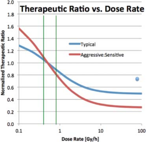 Figure 18.2. Relative Therapeutic Ratio as a function of dose rate, normalized to a dose rate of 0.5Gy/h. Each line assumes a particular ratio for the α and β in Equation 18.3 for tumor cells and normal cells. The blue line represents a typical situation, with α/β = 10 Gy for the tumor and 3 Gy for normal tissue. The red line applies to and aggressive tumor, with an α/β of 20 Gy and normal tissue with α/β or 2 Gy. The vertical green lines indicate the LDR region. The blue dot indicates the normalized therapeutic ratio for fractionated HDR treatments. |
Figure 18.2 illustrates the loss in therapeutic ratio with an increase in dose rate, and the loss in therapeutic ratio can be significant. Figure 18.2 also shows another interesting feature. The therapeutic ratio changes slowly with dose rate over the LDR portion of the curve (0.4–0.8 Gy/h, shown as green vertical lines in the figure), which accounts for historic LDR treatments giving similar results regardless of the exact dose rate. In that region, the therapeutic ratio does not change with absolute dose, only dose rate. At high dose rates, above 20 Gy/h, the therapeutic ratio again varies little with the actual dose rate. Most high dose-rate units deliver a dose at 1 cm at a rate of 100–500 Gy/h, but because much of an implant lies farther away than 1 cm at least some of the treatment time, the dose rate can fall well below that, but seldom below 12 Gy/h. Over any realistic HDR application, the dose rates anywhere in a volume of interest remain in the flat region of the curve. However, the biological dose distribution for an HDR application depends on the absolute dose level, and so differs from the physical dose distribution.
A very different situation obtains in the middle, transition region. In this case, the biological effectiveness of the radiation varies greatly with the actual dose rate, and the biological effectiveness of a given amount of dose varies with position in the treated volume. Often, treatments using nominally LDR remote afterloaders actually deliver doses at this middle dose-rate range. High precision is required with these devices to avoid exceeding tolerance of normal tissues.
The flat response in the HDR region of the curve traces back to the definition of “high dose-rate.” In Equation 18.3
the term α in the exponent does not depend on the rate of dose delivery. This term is often associated with single-track killing, that is, one charged particle passing near the DNA strand produces sufficient ionization in the right location to break both sides of the DNA “ladder.” Such a double-sided break can produce a biological effect, including cell death.2 The term β can be thought of representing the situation where the break on each side results from different charged particles. The cell can repair a single-sided break because the remaining side provides the template for the missing side. Tr, the half-time for repair of sublethal damage, characterizes this repair giving the time required to repair half of single-sided breaks. Measured values of Tr vary widely, but a typical value is 1 to 2 hours for both normal and tumor cells. Some normal tissues exhibit repair with two components, one with a half-time of approximately the value above but also a shorter component of about 20 minutes (7), although other models of repair kinetics fit the data better (8). Tumor cells seem not to have this faster component of repair, which gives another therapeutic advantage to the use of low dose rates. For the simple, single-component model for repair, the repair coefficient, μ, can be calculated as
the term α in the exponent does not depend on the rate of dose delivery. This term is often associated with single-track killing, that is, one charged particle passing near the DNA strand produces sufficient ionization in the right location to break both sides of the DNA “ladder.” Such a double-sided break can produce a biological effect, including cell death.2 The term β can be thought of representing the situation where the break on each side results from different charged particles. The cell can repair a single-sided break because the remaining side provides the template for the missing side. Tr, the half-time for repair of sublethal damage, characterizes this repair giving the time required to repair half of single-sided breaks. Measured values of Tr vary widely, but a typical value is 1 to 2 hours for both normal and tumor cells. Some normal tissues exhibit repair with two components, one with a half-time of approximately the value above but also a shorter component of about 20 minutes (7), although other models of repair kinetics fit the data better (8). Tumor cells seem not to have this faster component of repair, which gives another therapeutic advantage to the use of low dose rates. For the simple, single-component model for repair, the repair coefficient, μ, can be calculated as
Because the breaks repair over time, the probability for a second-sided break at the same location as the first depends how compact in time the radiation is delivered. When all the radiation passes through the DNA in a short period, the likelihood that the second side will break before the first side repairs increases compared with a long delivery. In this case, a “short” time relates to the half-time for repair of sublethal damage. Regardless of the actual dose rate, HDR treatment refers to a treatment where essentially all the breaks occur before any significant repair takes place. In general, HDR treatments should be completed within a half hour of commencement.
Fractionation
While reducing the dose rate is one method to improve the therapeutic ratio, another is fractionation. Figure 18.3 shows survival curves for the same parameters as Figure 18.1, but includes the survival curves for delivering the doses in 2-Gy fractions. The fractionation reduces the effectiveness of the radiation at killing cells, but it also reduces the differences between the responses of the tumor and the normal tissues.
HDR brachytherapy generally fractionates the treatment course to mitigate the problem of loss of therapeutic ratio with the increase in dose rate. Figure 18.4 shows the improvement in the therapeutic ratio by using one more fraction. For example, if a plan is called for the use of three fractions, the therapeutic ratio would improve by 4.7% by using four fractions instead. If five fractions were used instead of four, the therapeutic ratio would improve another 4% above the 4.7% improvement from increasing from three to four. As can be seen, each additional fraction improves the therapeutic ratio, but by less than the addition of the fraction before. In external-beam treatment, which is definitely HDR therapy, the number of fractions maybe 35, which would provide a great benefit in the therapeutic ratio, and the addition or deletion of one or two fractions would not make much a difference. Brachytherapy is both taxing on the patient and a drain on the personnel and resources
of the facility, and the use of a high number of fractions such as common in external-beam therapy, is not an option. Thus, a compromise must be made between improved therapeutic ratio and practicality. The number of fractions selected for curative cases depends on the amount of work involved and patient discomfort for each fraction. For interstitial cases with needle-like catheters in place, such as a prostate implant, three fractions are common. On the opposite extreme, breast implants with soft catheters and little patient discomfort often use 10, twice-a-day fractions. Intracavitary insertions involving the placement of a treatment appliance at each fraction often use five or six fractions. Tandem and ring applications using an indwelling Smit sleeve (a sheath for the tandem) in the uterine canal simplifies the procedure to the point to which 12 fractions have been used (9).
of the facility, and the use of a high number of fractions such as common in external-beam therapy, is not an option. Thus, a compromise must be made between improved therapeutic ratio and practicality. The number of fractions selected for curative cases depends on the amount of work involved and patient discomfort for each fraction. For interstitial cases with needle-like catheters in place, such as a prostate implant, three fractions are common. On the opposite extreme, breast implants with soft catheters and little patient discomfort often use 10, twice-a-day fractions. Intracavitary insertions involving the placement of a treatment appliance at each fraction often use five or six fractions. Tandem and ring applications using an indwelling Smit sleeve (a sheath for the tandem) in the uterine canal simplifies the procedure to the point to which 12 fractions have been used (9).
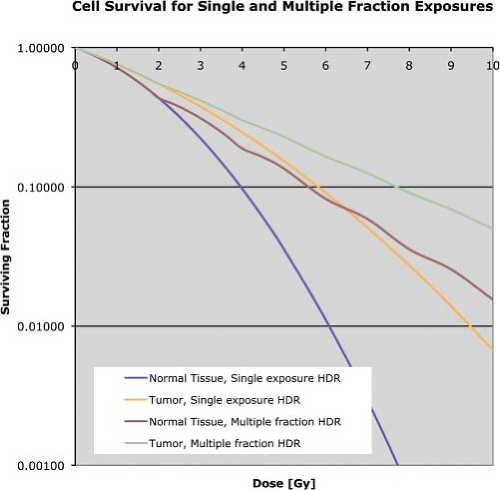 Figure 18.3. Survival curves using the same parameters as in Figure 18.1 for acute (single fraction) exposures and for 2-Gy acute fractions. |
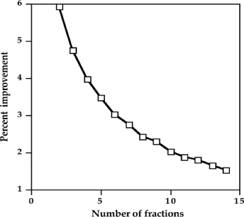 Figure 18.4. The percentage improvement in therapeutic ratio by the addition of one more fraction. |
Prescription Doses
Because the biological effectiveness of radiation changes going from LDR treatments to fractionated HDR treatments, the absolute dose prescribed also has to change to obtain the same therapeutic endpoint. As Equation 18.3 shows, cell survival has a more or less exponential relationship to dose, so dose proper is not the best variable to use when evaluating or predicting biological effects. Of several approaches, one of the most practical begins by taking the log of both sides of the dose response curves from Equation 18.3,
and then divided by -α to have at least the first term in dose alone, to give
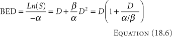
BED stands for biological equivalent dose. An equivalent term seen in the literature is the RDE, radiological dose equivalent. Equation 18.6 holds for acute, single exposures. For multiple HDR exposures of n fractions of d Gy/fraction, the BED becomes
Equation 18.7 holds when each fraction is short compared with the half-time for repair for cellular sublethal damage, and the time between fractions is long compared with this same half-time. As above, the duration of the treatment should be less than half hour, and the time between should be about 4 half-times, or about 6 hours. The newly included last term in Equation 18.7 gives the effect of cellular proliferation on the BED, where T is the total duration of the n fractions and Tpot is the potential doubling time for the cells. The equation shows that proliferation decreases the effectiveness of the radiation. This latter factor often is not known well; however, a compilation of values gleaned from the literature has recently been published (10). Conventionally, due to the uncertainty in this parameter, the proliferation is often ignored. For interstitial cases, the total therapy duration often remains the same; and therefore also the proliferation effect, whether the treatment chosen is HDR or LDR brachytherapy, as discussed below.
Protracted LDR therapy with some repair of sublethal damage taking place during treatment follows Equation 18.8 (11),
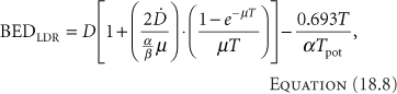
where [D with dot above] is the dose rate.
Assuming that the dose has been established for LDR treatments, the equation to produce the same biological effect with HDR brachytherapy can be calculated. The first step entails selecting the number of HDR fractions to use. As discussed above, this selection is an arbitrary compromise between improving the therapeutic ratio and practical utilization of resources. The next step sets the BED for each modality equal:
or
If the total times are similar, then the last terms on each side cancel. Even if they are not similar, since the values needed for their calculation are not well known, they often are simply ignored, giving
Table 18.1 Equivalent Treatments for LDR and HDR Brachytherapy | |||||||||||||||||||||||||||||||||||
|---|---|---|---|---|---|---|---|---|---|---|---|---|---|---|---|---|---|---|---|---|---|---|---|---|---|---|---|---|---|---|---|---|---|---|---|
| |||||||||||||||||||||||||||||||||||
BED depends on the tissue characteristics, as embodied in the values for α and β. Thus, the equivalence between LDR and HDR brachytherapy only applies to a single type of tissue—tumor or normal tissue. The dose cannot be equivalent for both simultaneously. An equivalent regimen must be selected to produce the same cure rate (equivalent for tumor) or the same normal-tissue reaction (equivalent for normal tissues). If the choice becomes too difficult, a compromise can be made—but at the cost of not being equivalent to the LDR regimen in any way. In general, making the HDR regimen equivalent to the LDR regimen for tumor tends to be the more common choice, since sacrificing cure rate would argue strongly against performing HDR brachytherapy, and physical techniques often can mitigate the increased effects on the normal structures. Early in HDR brachytherapy experience, Orton suggested that doses do not exceed 7 Gy/fraction to avoid normal tissue complications (12). The suggestion came from the review of a survey asking practitioners about their HDR experience. While the responses did indicate that complications increase with fraction sizes exceeding 7 Gy, the total doses for the cases in the survey were not controlled based on the linear-quadratic equations given here and commonly accepted in the present.
Complicating further the attempt to make an HDR brachytherapy treatment similar to one performed with LDR brachytherapy, notice that in Equation 18.12 the dose per HDR fraction, d, depends on the LDR dose to which it should be equivalent. This means that an HDR brachytherapy dose distribution can never be equivalent to an LDR brachytherapy dose distribution. Thus, to achieve a similar biological dose distribution, an HDR treatment should not duplicate the LDR physical dose distribution.
With interstitial implants, higher doses require more fractions to maintain normal tissues within tolerance doses. If the treatment catheters remain in place for the whole therapy, treatments frequently are given twice a day (BID). Table 18.1 relates LDR doses delivered at the rate of 0.5 Gy/h with the equivalent regimen with two HDR fractions per day. In general, the overall treatment duration—time with the catheters in place—remains about the same. The patient, however, need not be in radiation isolation with the HDR treatments.
For Intracavitary insertions, the prescribed dose often falls at an unambiguous (although often arbitrary) location, for example, Point A for cervical cancer, the surface of a cylinder for vaginal cancer, or 1 cm from the center of the applicator for esophageal applications. Interstitial implants are sometimes less well determined. Take, for example, a post-tylectomy breast implant with a seroma visible on computer tomography (CT). The clinical target volume (CTV) might be the seroma plus a 1.5-cm margin, limited to remain 5 mm deep to the skin and not enter the pectoralis major. During the dosimetry process, the prescription-dose (100%) isodose surface ideally is set at the CTV. All these seem very straightforward. However, depending on where the source tracks fall with respect to the CTV, the 100% isodose may lie on the edge of the more or less uniform dose plateau of the implant or in the rapidly decreasing gradient. (It should be assumed that the 100% isodose surface would never fall beyond the rapidly decreasing gradient to where the dose decreases more slowly; that would be a poor plan indeed.) Thus, in actual cases, some of the CTV may not receive the full dose and some of the prescription isodose surface may fall outside the CTV. Some guidelines for specifying the prescription dose are given in the section on “Evaluation.”
Optimization
In brachytherapy, “optimization” generally connotes determination of some aspects of an application in order to achieve particular goals. For example, optimization may have as a goal delivering a minimum dose to a target volume with a specified homogeneity. With permanent implants of the prostate, optimization usually generates a pattern for locations of the sources to deliver 90% of the prescription dose to the entire CTV,3 limit the volume raised to 300% of the prescription dose, and avoid doses to the rectum and
urethra that exceed their respective tolerances. In HDR brachytherapy, the most common optimization process determines the dwell times that produce the desired dose distribution—rarely does the process determine catheter location which usually is given. The assumption is that the planning of the implant, that is, where catheters or appliances should lie, occurs at a previous stage. This forms the basic difference between the HDR brachytherapy and the permanent implant cases—for permanent implants, optimization is a part of planning, while for HDR brachytherapy optimization is simply a part of dose computation.
urethra that exceed their respective tolerances. In HDR brachytherapy, the most common optimization process determines the dwell times that produce the desired dose distribution—rarely does the process determine catheter location which usually is given. The assumption is that the planning of the implant, that is, where catheters or appliances should lie, occurs at a previous stage. This forms the basic difference between the HDR brachytherapy and the permanent implant cases—for permanent implants, optimization is a part of planning, while for HDR brachytherapy optimization is simply a part of dose computation.
The optimization problem in HDR brachytherapy tends to be simpler than for permanent implants with a single source strength, and can usually come closer to achieving the goals of the optimization. While the permanent implant problem can only decide whether or not to place a source in a given location, the HDR brachytherapy problem can begin assuming activation of all possible dwell locations, and then simply determine each dwell time. Sometimes, the easiest approach determines the dwell times relative to either the maximum time or some specific time (dwell weights) for each dwell position in order to achieve some uniformity, and then set the times in proportion to the dwell weights required for the dose. If solution for the problem does not require a particular dwell position, the optimization routine (optimizer) needs only set the weight to zero. There are several, very different approaches to optimization. Ezzell (13), and Ezzell and Luthmann (14) present excellent discussion on optimization theory and characteristics.
The optimization problem usually specifies a goal. A simple goal might be to deliver a particular dose to a particular location. More specific goals might include delivering the same dose to a set of points or a surface. Even more complex goals not only specify the dose to a surface, but the homogeneity of the dose through the bounded volume and maximum doses allowed to neighboring sensitive normal structures. With the more involved goals, one of the features of the optimization approach includes how to specify the problem and determine the importance of all the varied, and often conflicting, requirements. Many of the optimization approaches use an objective function to wrap all the goals into a single measure. And example of an objective function, OF, for a prostate implant could be
where D stands for doses and w for weighting for the term. The first term considers the target voxels, denoted by subscript t. The first goal would be to deliver the prescribed dose to the target. Any voxels falling below the prescribed dose would add to the objective function. Homogeneity, indicated by the subscript h, also applies to the target voxels, and in the second term, voxels exceeding twice the prescribed dose add to the OF. The last two terms address dose to the rectum and urethra, and increase the OF for voxels that exceed a specified limit for the respective organ. The goal of an optimization could be to minimize this objective function. Objective functions (sometimes called cost functions) can be simpler or more complicated, and can be set such that the goal may be to minimize or maximize the function.
Considering the function above, there maybe many combinations of dwell times that satisfy all the requirements, so there would not be a unique solution. In the subset of all solutions, some may be better than others. If the differences in solutions make a difference in the perceived quality of the treatment plan, then the objective function should be modified to reflect the additional requirements or tighten the specifications. If the differences in the solution remain unimportant, then the first solution found could be used.
While there are many approaches to optimization, they tend to fall in general categories. The actual distinctions between the categories seldom are as clear as it seems they should be, and into which category a given approach falls often remains debatable. Nevertheless, the discussion below considers the characteristics of some of the major categories.
Deterministic Approaches
Deterministic approaches to optimization always find the same solution to the same problem, and generally solve equations to find the dwell times.
Heuristic Approaches
Heuristic approaches use pragmatic search techniques to construct solutions to the optimization problem. The search techniques may use surrogates for the optimized quantities if they are useful. Optimization purists might maintain that heuristics are not true optimization approaches because they tend not to produce a true optimum but merely a satisfactory result. For clinical problems, satisfactory results often serve the patient needs well. In any case, the results of the optimization must be evaluated for appropriateness.
For HDR brachytherapy, one of the most widely used heuristic approach is geometric optimization, developed by Edmundson (15). Geometric optimization assumes the goal is a uniform dose distribution, and further assumes a distribution of dwell positions through the volume to receive the uniform dose. The first step in the optimization process recognizes that the dose to the region of the target around a dwell position results not only from
the radiation emanating from that dwell, but from all the other dwell positions as well. Looking first at what dose is received at a given dwell position from all the other dwell positions, the weighting of the dwell under consideration should be inversely proportional to the dose from the other positions. Thus, dwell positions that receive large doses from the other dwell positions should have shorter dwell times and those with little contribution from other dwells should have long times. Mathematically,
the radiation emanating from that dwell, but from all the other dwell positions as well. Looking first at what dose is received at a given dwell position from all the other dwell positions, the weighting of the dwell under consideration should be inversely proportional to the dose from the other positions. Thus, dwell positions that receive large doses from the other dwell positions should have shorter dwell times and those with little contribution from other dwells should have long times. Mathematically,
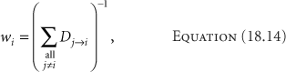
where Dj→i is the dose from dwell position j delivered to dwell position i. The commercial versions of the programs approximate Dj→i with the inverse square relationship, using Equation 18.15,
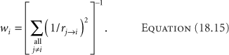
Such an approximation is expedient but not necessary.
One problem with geometric optimization in the form of Equation 18.14 is that the optimization assumes equal dwell times during the calculation of the dwell weights, but then uses the calculated weights for the treatment. Thus, the treatment does not match the conditions for the optimization. This problem could be rectified through an iterative procedure, where the dwell weights for current iteration used those calculated in the last, such as
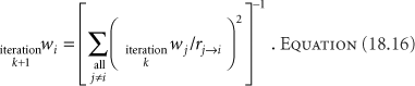
The iteration would continue until the dwell weights changed less than some specified percentage. Geometric optimization tends to underweight the periphery of implanted volumes. The iterative procedure could rectify this shortcoming.
A refinement of the approach ignores the contribution of those dwell positions within a specified radius of the one being calculated, assuming that the influence of very close dwells may unduly influence the resultant weights. Applying this technique of ignoring the nearby dwell positions goes by the name volume optimization. In practical implementation, often the calculation of the dose to a dwell position ignores the contributions from dwells along the same catheter track. When optimizing few source tracks, such as single catheters for esophageal treatments or a tandem and ovoid, all dwell positions would be included in Equation 18.14—a process then known as distance optimization.
Convergent Searches
Also called “downhill searches,” convergent searches minimize the objective function iteratively (16,17). At each iteration, the program decides which direction to make changes and how much change to make, based on the differential of the objective function with respect to the parameter being optimized in that pass. These methods tend to get stuck in local minima if they occur between the starting condition and the true minimum. At the time of writing, no commercial brachytherapy planning system uses this technique, although given the popularity of downhill searches in optimization for intensity-modulated radiotherapy the method may move into HDR brachytherapy.
Point-Dose Optimization
Geometric optimization works without reference to an actual dose distribution. Point-dose optimization forms the most direct optimization approach actually to address doses. For this approach, the operator specifies doses to deliver to particular points (optimization points). The process then straightforwardly establishes a set of equations for the doses to the optimization points, of the form
where fi→a denotes the function that describes the dose at optimization point a resulting from the source at dwell position i per unit dwell time. The dwell time, ti, becomes the unknown in the equation. Each optimization point forms one equation, and each dwell time an unknown. Together they form a set of simultaneous equations. Unfortunately, solution of the set of equations presents two problems. The first problem is nonphysical solutions. Consider the situation with the same number of unknown dwell times and optimization points—a determined system. For a very simple case as shown in Figure 18.5 with 12 dwell positions, separated by 1 cm, and 12 optimization points, where each point falls 3 cm above the dwell position.
Further, to simplify the problem, approximate the source as a point so the dose rate only depends on the source strength, SK, the dose-rate constant, Λ, and the inverse of the distance, r. (For 192Ir the other factors are minor and could be ignored for the example.) Assume that all the optimization points should receive the same dose. The system of equations becomes
Further, to simplify the problem, approximate the source as a point so the dose rate only depends on the source strength, SK, the dose-rate constant, Λ, and the inverse of the distance, r. (For 192Ir the other factors are minor and could be ignored for the example.) Assume that all the optimization points should receive the same dose. The system of equations becomes
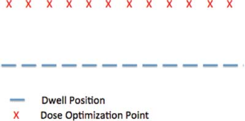 Figure 18.5. An example for optimization: a single catheter with 12 dwell positions at 1 cm intervals, and 12 optimization points, each 3 cm below every dwell position. |
where every Di = the dose at point i = the prescribed dose, and j indicates the source dwell position. Solving this system gives relative dwell weights of:
1.00, 0.08, -0.18, 0.26, 0.50, -0.02, -0.02, 0.50, 0.26, -0.18, 0.08, 1.00.
The negative dwell weights are necessary to satisfy the dose requirements. Simply deleting those dwell times, or increasing all the times by the amount of the most negative fails to produce the uniform dose.
A method to deal with the potential negative values for the dwell times developed by van der Laarse adds a constraint to reduce the variation between adjacent dwell times (18). With control of the variation of dwell times, the equation for optimization becomes
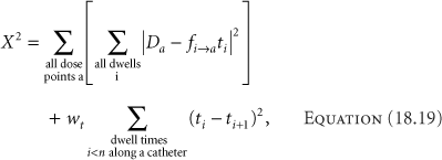
where wt is the dwell-time gradient weighting factor, a measure of the importance of minimizing the differences between adjacent dwell times, and n is the number of dwell positions along a catheter. The first term aims to minimize the differences between the desired doses at the optimization points and the calculated doses. The optimization process then becomes minimizing the chi-square, χ2. Delivery of any dose requires the net dwell time summation to be positive, so there is no concern that the process might yield all negative times. Minimizing the differences between adjacent dwell times only makes sense locally, that is, along a catheter. Each catheter starts a new comparison of times. The best correlation between desired and calculated doses comes with the smallest value of wt that eliminates negative dwell times. The values for wt have no limiting range, although increasing the value above approximately 0.8 has little effect on the dose distribution.
Adding a dwell-time gradient control factor to the problem in Figure 18.5 and Equation 18.19 produces the dwell weight pattern of:
1.00, 0.31, 0.04, 0.10, 0.37, 0.22, 0.22, 0.37, 0.10, 0.04, 0.31, 1.00.
All the dwell weights have become positive. The value for the dwell weight gradient control factor in this example was just 0.01. A small amount of control makes a marked difference. The uniformity suffered slightly in this case. With the negative dwell weights, the dose at the end optimization points fell -4% below the average dose to the points, but the remaining points were within ±1%. With the control of the dwell times, the end points improved to -3%, but the rest of the points varied between -1% and +3%. The results of any optimization always require evaluation to assure that the clinical needs are met.
Approaching the problem as a minimization of chi-square also addresses another problem. While the single catheter example above had the same number of dwell positions and optimization points, real cases often have more dwell position than optimization points (making an underdetermined system of equations) or fewer (overdetermined)—either posing a situation that cannot be solved exactly just by manipulating the equations. The chi-square approach gives the best approximation to a solution. Underdetermined cases have many possible solutions. A useful criterion for selecting the best of the solutions controls the overall treatment time. While simply selecting the solution that minimizes the sum of the dwell times provides a straightforward method to achieve this, minimizing the sum of the squares of the dwell times tends to provide a more uniform distribution of dwell times, and likely of dose (19).
The results from optimization algorithms always need evaluation. The algorithms, of course, do what they are instructed, but the instructions may not be exactly the operator’s intention. Consider the simple example of three dwell positions around a point, as shown in Figure 18.6, based on an example of van der Laarse. Point optimization simply specifying the dose to the point could result in the use of only one of the dwell positions, when the intention probably was to use all three and cover a larger volume. Either using a high value for the dwell-time gradient weighting factor or adding optimization points at locations where the dose is actually desired would solve the problem.
A further reason to review the results of the optimization carefully is that the optimization requirements may not have a solution. The line problem of Figure 18.5 had no solution that produced the prescribed dose at each of the optimization points. Depending on the problem, the solutions may be close to the specifications or not. Particularly for underdetermined problems, where the
number of optimization points exceeds the number of dwell positions, the probability of obtaining the desired dose at all points becomes low. Evaluation procedures are covered in the section on “Evaluation.”
number of optimization points exceeds the number of dwell positions, the probability of obtaining the desired dose at all points becomes low. Evaluation procedures are covered in the section on “Evaluation.”
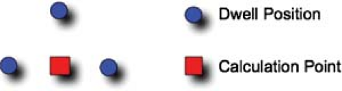 Figure 18.6. Three dwell positions around a point, based on an example case from van der Laarse. |
Modern brachytherapy, as with external-beam radiotherapy, tends to specify doses to the surface of a target volume rather than a few points. Programs often approximate surfaces with a collection of closely spaced points. Controlling the dose within a volume often requires more points. This proliferation of optimization points (equations) takes a greatly increased amount of computer resources. Direct algebraic approaches become less appealing.
Polynomial Optimization
A typical (not large) interstitial implant may have 25 catheters, each with 15 dwell positions, resulting in a total of 375 dwell positions. As noted at the end of the last paragraph, the number of optimization points in this case may also become exceedingly large—likely approximating the number of dwell positions. Thus, the system could have 375 equations—each with as many unknowns. This could take some time to solve. Van der Laarse proposed that with the dwell-time gradient weighting factor, the dwell times in a catheter could be constrained to the point that a polynomial could describe their pattern (19). The advantage of fitting the dwell times along a catheter is the reduction in parameters from the number of dwell times to the fitting parameters. Van der Laarse suggests that for n dwell positions in a catheter, a polynomial of order p could model the dwell times, where
Using the polynomials, the dwell time at position i along a catheter, at the distance xi from the beginning of the catheter, becomes
The optimization then substitutes Equation 18.21 in Equation 18.19, and sets  to find the optimum fit for the polynomials. to find the optimum fit for the polynomials. |
Polynomial optimization as implemented in the Nucletron4 planning systems uses geometric optimization to give a first-pass value for the dwell times for volume implants, sums the resulting dwell times along each catheter, and divvies that time to each dwell position in proportion to the values resulting from Equation 18.21 divided by the total of the ti(xi) for the given catheter.
Related posts:

Stay updated, free articles. Join our Telegram channel

Full access? Get Clinical Tree


