Fractionation: Radiobiological Principles and Clinical Practice

Colin G. Orton

Introduction

From the very beginning of radiotherapy, treatments were fractionated. For example, on January 29, 1896, just 1 month after Roentgen announced his momentous discovery of x-rays to the world, Emil Grubbé in Chicago was reported to have begun administration of a course of 18 daily 1-hour fractions of radiotherapy to a patient with cancer of the breast (1). More fractions would have been delivered, but treatment had to be terminated when the patient developed a virulent dermatitis. Within a few years, hundreds of patients had been treated with fractionated radiotherapy worldwide.

In these early years just about all radiotherapy was fractionated, but fractionation was used not because it was known that this was the appropriate way to deliver high doses without exceeding normal tissue tolerance—as we know today—but because of the very low output from the early x-ray machines available at that time. To deliver a single dose sufficient to destroy a tumor would have required several hours—sometimes even days—so treatments had to be given in several sessions. Single-fraction radiotherapy did not become feasible until 1914 with the advent of the Coolidge hot cathode tube, with its high output, adjustable tube current and reproducible exposures. The ensuing two decades witnessed a period of uncertainty as to the proper way to fractionate. Reportedly, there were two schools of thought: Erlangen and Paris (2). Wintz, from Erlangen, led a group of radiotherapists who believed that single doses were necessary to cure cancer, and they referred to fractionated treatment as “decisively inferior and … to be considered weak irradiation or the primitive method.” Their rationale for single-fraction radiotherapy was based on their interpretation of the Bergonié–Tribondeau Law of radiation sensitivity, published in 1906, which concluded: “From this law, it is easy to understand that roentgen radiation destroys tumors without destroying healthy tissues.” Therefore, it appeared that there was an inherent advantage of roentgen irradiation that might be lost if cancer cells were allowed time to recover. Wintz and his colleagues argued that “recovery from radiation injury depends on cellular metabolism and a rapidly growing tumor cell is better able to affect recovery from injury than a connective tissue cell. Therefore, the difference in recovery will favor the tumor if the cancerocidal dose is not applied in the first treatment” (1).

The Paris School, on the other hand, used the radiobiological experiments of Regaud on the effect of fractionation on the sterilization of rams to justify the need to fractionate. Regaud found that it was possible to sterilize rams by irradiation of their testes without excessive damage to the skin of the scrotum only if the treatments were fractionated. When single doses were given, such sterilization was possible only with induction of unacceptable skin damage. Regaud postulated that the testes could be considered a good model to simulate a rapidly dividing cancer and, therefore, fractionation ought to allow a cancerocidal dose to be delivered without exceeding normal tissue tolerance. This led to a careful study of fractionated radiotherapy by Henri Coutard at the Curie Institute in Paris (2).

The debate over fractionation was not settled until 1932, when Coutard published the excellent results he had obtained using fractionated radiotherapy (3). Fractionation was thereafter established as the standard of practice of radiotherapy. However, it is only relatively recently that the radiobiological rationales for fractionated radiotherapy have been fully understood.

Radiobiological Principles of Fractionation

The basic principle of radiotherapy is the destruction of all cancer cells without killing so many normal cells as to exceed tolerance. Thus, cell survival and the shape of cell survival curves is of utmost importance in radiotherapy.

Cell Survival Curves

A plot of the fraction of surviving cells as a function of dose for acutely irradiated cells is shown in Figure 21.1. Note that surviving fraction is plotted on a log scale. This is partly because, as we will see later, the shape of the log-linear survival curve for specific cell types tells us something about the important radiobiological properties of these cells, and partly because much of the important information about cell survival is contained within the low and high dose extremes of the survival curve (regions A and B in Fig. 21.1). Plotting cell survival on a log scale helps us visualize and
study the shape of the survival curve in these regions. It is low doses per fraction (in region A) that are used for fractionated radiotherapy (1–3 Gy/fraction) and, to cure a tumor with typically 10⁸ to 10¹⁰ cells, cell-surviving fractions as low as 10^-8 to 10^-12 are required (region B).

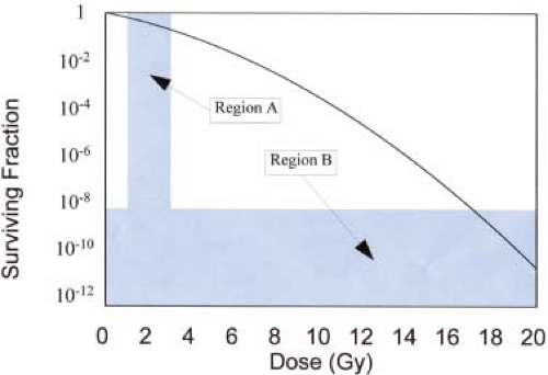Figure 21.1. Graph showing the surviving fraction of cells (log scale) as a function of dose. The two shaded areas represent the regions of most interest in fractionated radiotherapy for which doses per fraction normally range from 1 to 3 Gy (region A) and the cell-surviving fraction required to control a typical tumor containing 10⁸ to 10¹⁰ cells must be on the order of 10^-8 to 10^-12 (region B). This hypothetical graph has been constructed according to the linear quadratic (LQ) model with parameters α = 0.4 Gy^-1, α/β = 10 Gy.

Since the shapes of cell survival curves are so important, it is necessary to have a mathematical model that can predict these shapes. Currently, the model of choice is the linear quadratic (LQ) theory of cell survival.

Linear Quadratic Theory

The basis of the LQ theory is that a cell is inactivated only when both strands of a deoxyribonucleic acid (DNA) molecule are damaged. Actually, this is a gross oversimplification of the highly complex chemical and biological responses triggered by irradiation of cells, but this was the basic assumption made when the LQ model was first devised (4) so, for simplicity, we will adopt this approach here. Readers interested in a more thorough (and accurate) discussion of the complex events that occur when cells are irradiated are referred to an excellent review by Wouters and Begg (5).

On this simple model, double-strand breaks can be produced either during the passage across the cell of a single ionizing particle or by independent interactions by two separate ionizing particles. Such events are random and, because there are large numbers of cells, the probability that any specific cell will be inactivated will be extremely low. Under such conditions, the statistics of rare events (Poisson statistics) prevails. According to Poisson statistics, the probability of there being no such lethal events, that is, the surviving fraction, S, of cells, is given by the expression (6):

where p is the mean number of hits per cell. For single-particle events, p is a linear function of dose, D, so the mean number of hits/cell can be expressed as αD. Then, Equation 21.1 can be written as:

where α is the average probability per unit dose that such a single-particle event will occur. In order for a single particle to damage both arms of the DNA in a single passage across the molecule, it has to be fairly densely ionizing, that is, high linear energy transfer (LET). With photon and electron irradiation, it is only the slow electrons that are responsible for most of these interactions. Conversely, when cells are irradiated with high-LET radiations, such as α-particles and heavy ions, almost all the events will be by single particles, so cell survival will be governed by Equation 21.2 and cell survival curves will be practically linear.

For the two separate ionizing particle events of the LQ theory, the mean probability of one particle causing damage in one arm of a DNA molecule in any specific cell is linearly proportional to dose, as also is the mean probability that a second particle will have such an interaction in the adjacent arm of this same DNA molecule. Therefore, the mean probability of both events occurring is βD ², so the probability that no such two-particle events will occur is given by:

where β is the mean probability per unit square of the dose that such complementary events will occur.

The overall LQ equation for cell survival is therefore:

This is illustrated in Figure 21.2, which shows how the two components of cell killing, α-damage and β-damage, combine to form the cell survival curve. It will be shown later that α-damage and β-damage relate to irreparable and repairable damage, respectively. For two-particle
events (β-type), if the damage from the second particle occurs before the lesion from the first particle has been repaired, the cell will be inactivated (“killed”). Since cellular repair half-times are of the order of 1 hour, this gives rise to the dose-rate effect: the higher the dose rate, the greater the effect.

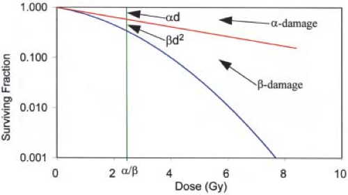Figure 21.2. Linear-quadratic cell survival curve, with α = 0.22 Gy^-1 and α/β = 2.5 Gy. Note that the log cell kill for α-type damage equals that for β-damage at a dose equal to α/β.

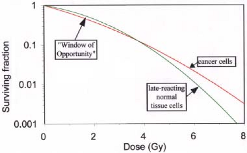Figure 21.3. Typical survival curves for cancer and late-reacting normal tissue cells, superimposed for comparison. Compared with the cancer curve, the normal tissue cell survival curve has a shallower initial slope (lower α) and is “curvier” (lower α/β). Note that there is a “Window of Opportunity” below ∼4 Gy (with the parameters used here) where normal tissue cells exhibit a higher survival than cancer cells. Parameters used to draw these hypothetical curves are as follows: tumor, α = 0.4 Gy^-1, α/β = 10 Gy; late-reacting normal tissues, α = 0.22 Gy^-1, α/β = 2.5 Gy.

Of special interest is the dose at which the log-surviving fraction for α-damage (-αD) equals that for β-damage (-βD ²), that is, αD = βD², or D = α/β. This is also illustrated in Figure 21.2. This parameter, α/β, represents the curviness of the cell survival curve. Specifically, the higher the α/β, the straighter the curve. Similarly, a high α/β is characteristic of a type of cell that exhibits considerable irreparable damage and/or little repair (high α and/or low β). In contrast, a low α/β (low α and/or high β) indicates little irreparable damage and/or a high capability of repair. Here lies the major difference between the cells of tumors and those of late-responding normal tissues: α/β values tend to be high for cancers and low for late-reacting normal tissues. For example, typical α/β values determined for cancer cells range from 5 to 20 Gy (mean ∼10 Gy), but for late-responding normal tissues the range is 1 to 4 Gy (mean ∼2.5 Gy). There appear to be some exceptions, however. For example, the α/β values for prostate and breast cancer cells have been reported to be about 1.5 and 4 Gy, respectively (7,8).

Figure 21.3 shows typical survival curves for tumor and late-reacting normal cells, superimposed for comparison. The difference in the shapes of cell survival curves of cancer and normal cells provides the major rationale for fractionated radiotherapy.

Rationale for Fractionation

Radiotherapy, in general, is governed by the four Rs: repair, reoxygenation, repopulation, and redistribution, and so also is fractionation. Following is a discussion of how each of the four Rs affects the practice of fractionation.

Repair

Of all the four Rs, repair is the most important in terms of the rationale for fractionation. As discussed in the preceding section, late-reacting normal tissue cells tend to exhibit a greater propensity for repair than do tumor cells. This is exhibited by their low α/β values and their curvier survival curves, as shown in Figure 21.3. In this illustration, the normal tissue and tumor cell curves cross at doses of the order of 4 Gy. At doses below the crossover point, cell survival for late-reacting tissues is greater than that for tumors, and the reverse is true above the crossover. This means that delivery of doses greater than ∼4 Gy will be more destructive to normal tissues than to cancer cells. There is essentially a “Window of Opportunity” centered at ∼2 Gy within which normal cells have a greater survival than cancer cells. However, doses far in excess of 4 Gy are needed to control tumors. There are two ways to safely deliver such high doses. One is to deliver much higher doses to the tumor than to the normal tissues, such as with stereotactic radiosurgery (SRS), intensity-modulated radiation therapy (IMRT), and various other forms of conformal therapy. This will be discussed in detail later. The second option is to fractionate with doses/fraction within the “Window of Opportunity.”

If a course of fractionated radiotherapy is delivered with time between fractions sufficient for complete repair (which clinical evidence has shown to be about 6 hours or more), all the cells that have been sublethally (but not lethally) damaged during the first exposure will have repaired before the second, and so on. This relates to the β-type damage in the LQ model. Then, at least to a first approximation, cell-surviving fractions for each successive treatment will be identical, that is, the shape of the survival curve will simply repeat for each fraction and the cell-surviving fraction equation becomes:

where N is the number of fractions and d is the dose/fraction. Then, if the dose per fraction is below the crossover point shown in Figure 21.3, the resultant cell survival curves gradually separate, with tumor cells suffering more damage than normal cells, as illustrated in Figure 21.4, which has been derived using Equation 21.5.

At least as far as repair is concerned, the optimal dose per fraction is that, which will produce the maximum separation of the two fractionated radiotherapy curves in Figure 21.4. However, the LQ model predicts that this maximum separation occurs with an infinite number of infinitely small dose fractions, each separated by sufficient time for complete repair. Clearly, this is not a realistic fractionation scheme, and in any event it ignores the influence of the other three Rs of radiotherapy, especially repopulation (see later discussion). With this in mind a better
definition of the optimal dose per fraction is where the rate of increase in separation of the two fractionated radiotherapy curves in Figure 21.4 per unit number of fractions is a maximum. It can be shown that this occurs at the point of maximum separation between the acute exposure tumor and normal tissue curves shown in Figure 21.3, which turns out to be at exactly 50% of the dose at the crossover point. For the parameters used to plot the survival curves in Figure 21.3, this dose is ∼2 Gy. Hence, the optimal dose per fraction is about 2 Gy. If the α and β values for normal tissues and tumor were known for each patient, it would be possible to design patient-specific fractionation regimens but, unfortunately, the technology to do this is not refined enough at present. The alternative is to determine the optimal dose per fraction for specific types of disease for the average patient, and this has been the objective of numerous clinical trials of altered fractionation (2,7,8,9,10,11,12,13,14,15,16,17).

Figure 21.4. How fractionation with dose per fraction below the crossover point of the late-responding normal tissue and tumor cell survival curves in Figure 21.3 results in higher cell survival for the normal tissue cells as the total dose increases.

The situation is somewhat different for SRS and other forms of highly conformal radiotherapy, because the effective dose to normal tissues is usually kept well below that to the tumor, where the “effective dose” may be defined as the dose that, if delivered uniformly to the tissue in question, would result in the same probability of local control or complication as the actual inhomogeneous dose distribution in that tissue. Several methods to determine such effective doses from dose–volume data have been published (18,19,20,21,22,23,24) and these are reviewed in Chapter 23. For example, if f (the geometrical sparing factor) is the ratio of the effective dose in normal tissues to effective dose in tumor, even a modest sparing represented by f = 0.8 moves the crossover point to considerably higher doses and significantly widens the “Window of Opportunity,” as shown in Figure 21.5. In this example, the crossover point moves from 4 Gy all the way out to about 14 Gy, so the optimal tumor dose per fraction becomes ∼7 Gy. Interestingly, this is the typical tumor dose per fraction used for high dose-rate brachytherapy for cervix cancer, with which significant geometrical sparing inherent with the brachytherapy modality can be expected.

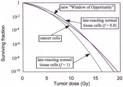Figure 21.5. How the crossover point for single (acute) irradiations shown in Figure 21.3 moves to considerably higher tumor doses if there is even a modest amount of “geometrical sparing” of the normal tissues (the normal tissue curve moves 20% to the right). In this example, a 20% sparing (f = 0.8) causes the crossover point to move from ∼4 Gy out to 14 Gy. The same linear quadratic (LQ) model parameters as for Figure 21.3 are used here.

For SRS, single doses of the order of 20 Gy are used. It is readily shown that with the parameters used to plot Figures 21.3 to 21.6, this will be optimal if f equals ∼0.6, not too unlikely, especially for small tumors. For large tumors, f may exceed 0.6, so fractionated radiotherapy might be required.

One concern with SRS and other types of radiotherapy such as IMRT, CyberKnife, and so on, for which the time it takes to deliver a treatment session can be of the same order of magnitude as the half-time for cellular repair, is that repair during irradiation might reduce the effectiveness of the treatment. Studies have shown that this effect might cause reductions in effective dose as much as about 12% if the time to deliver the treatment is as high as about 0.5 hours, with concomitant reductions in tumor control as much as 30% (25). Fortunately, it is possible that protraction of irradiation time during a treatment might reduce the effect on normal tissues more than on cancers (26). Hence, it might be possible to increase the total dose sufficiently to offset the effect of this intrafraction repair without increasing the damage to normal tissues.

All the foregoing discussions, and especially the dose per fraction estimates, are of course highly dependent on the α and β parameters assumed. They also totally ignore the effect of the other three Rs of radiotherapy.

Reoxygenation

Oxygen is the most powerful of all radiation sensitizers, so cells deprived of oxygen are relatively resistant to radiation and require approximately three times as much dose as well-oxygenated cells to destroy them. Such doses in a course of radiotherapy will likely exceed normal tissue tolerance unless highly conformal therapy is used. Furthermore, there is evidence that a significant proportion of human cancers contain hypoxic cells (27,28,29,30,31,32). It would be
expected, therefore, that immediately after the exposure of a tumor to radiation, the fraction of the surviving cells that are hypoxic should increase because the sensitive, well-oxygenated cells will be killed preferentially. Indeed, this is exactly what has been observed in many animal in vivo experiments. However, in some of these experiments, the hypoxic-cell fraction rapidly returned to the much lower pre-irradiation levels, and this has been interpreted as reoxygenation (33). In that case, if enough time is allowed for reoxygenation between exposures in a course of fractionated radiotherapy (typically 24 hours is sufficient), the number of hypoxic cells in a tumor reduces to a level that can be handled by doses that do not exceed normal tissue tolerance. Hence, fractionation takes on added importance when treating tumors with a significant hypoxic-cell fraction. However, there is some evidence that fractionation does not always ensure sufficient reoxygenation to overcome hypoxic-cell radioresistance. For example, several clinical trials have demonstrated that pre-irradiation hypoxia significantly reduces local control even after an extended course of fractionated radiotherapy long enough to ensure reoxygenation (27,28,29,30,31,32). If complete reoxygenation were taking place between fractions, such reductions in local control would not be expected.

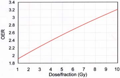Figure 21.6. Illustration of the increase in oxygen enhancement ratio (OER) with increase in dose/fraction. Parameters used (see text) are those derived to fit clinical data for the treatment of prostate cancers by Nahum, et al. (30).

Another aspect of the effect of oxygen on fractionated radiotherapy relates to the effect of LET. When cells are exposed to high-LET radiation, the protective effect of hypoxia is greatly reduced (33). Hence, in the part of the cell survival curve where α (i.e., high-LET) damage predominates, that is, at low dose or low dose/fraction (see Fig. 21.2), the effect of hypoxia should be less than where β-damage predominates, that is, at high dose or high dose/fraction. This effect of dose or dose/fraction has been demonstrated by cell survival experiments (34,35) and has been shown to be consistent with clinical data (30).

Only gold members can continue reading. Log In or Register to continue