3 Fractionation Effects in Clinical Practice
Radiation dose fractionation—the temporal programming of radiation delivery—has been a fruitful field of clinical research throughout the history of radiation therapy and has been one of the main arenas for attempting to improve the therapeutic ratio.* With the further development and wider use of the linear-quadratic (LQ) bioeffect formula around 1980 and its success in explaining a flurry of clinical and experimental fractionation data during the next decade or so, many clinical radiation researchers believed that the main effects of dose fractionation on tumors and normal tissues were finally well understood; everything that could be discovered had been discovered, and it was only a question of time before the last outstanding problems were cleared away. Interestingly, the whole field of clinical fractionation research has undergone a veritable renaissance since then, and there seems to be even more research challenges and opportunities today than there were back in the 1980s and 1990s. This revived interest has been stimulated by the introduction of new treatment planning and delivery technologies during this period. In addition, the wider use of combined treatment modalities has reopened many questions relating to optimal dose fractionation. But more than anything, a large body of clinical and biologic research has challenged many of the dogmas taught just 10 or 15 years ago. Although much of the teaching of dose fractionation biology has traditionally relied on assumed parallelisms between humans and a variety of biologic model systems, the discussion can now largely be based on clinical data from case series or even from randomized controlled trials. In this chapter, results of randomized trials are cited whenever relevant, but, rather than tabulating a long string of individual trials, the focus of this chapter is on using and understanding the biologic insights derived from clinical studies.
Conventional and Altered Fractionation
The Origins of Conventional Fractionation
Within a few years after Röntgen’s discovery of x-rays in 1895, the first attempts were made at using these new rays in the treatment of benign and malignant disease and the first cures of human skin cancer with radiation therapy were reported independently by two Swedish physicians, Tage Sjögren2 and Thor Stenbeck,3 in 1899 and 1900. It became almost immediately clear that the biologic effects of a given physical absorbed dose depend strongly on the details of how this dose is delivered over time. As early as in 1902, Ludwig Teleky recommended dose fractionation as a means of reducing the level of late side effects in a discussion in the Royal Society of Physicians in Vienna.4
With advances in x-ray technology, it became technically possible to deliver a large enough dose to produce a visible skin reaction in a single sitting. Biologic reasons for preferring short, intensive schedules were mainly speculative rather than based on empirical data, but these schedules won many supporters especially in Germany and Sweden. A few systematic experimental studies tried to compare single dose versus fractionated radiotherapy for various tissues. In 1927, Regaud and Ferroux showed that it was possible to sterilize a ram’s testis without excessive skin reactions using fractionated radiation but not using single doses,5 experiments that have become part of radiotherapy folklore. Regaud proposed, controversially at the time of publication, that spermatogenesis could serve as a model of human cancers. We now know that the “inverse fractionation effect” he observed (i.e., a larger effect with decreasing dose per fraction [F]) is unique to the spermatogenic system. What Regaud did realize was that it is not the biologic effect of higher dose per fraction in itself than matters, but rather the differential effect of changes in dose per fraction for tumors and the relevant normal tissues. Jens Juul in Denmark experimented on transplantable murine tumors in the late 1920s and used skin as the relevant normal tissue in a series of studies based on the idea of treating to isotoxicity6 and concluded that fractionated radiotherapy yielded a superior therapeutic index. For a more detailed account of these studies, see Bentzen and Thames.7 The fractionation debate was finally settled by clinical observations and by the early 1930s there was a widespread consensus that curative radiation therapy should be delivered in multiple fractions (so-called fractionated-protracted radiotherapy) rather than as a large single dose. What is even today referred to as conventional fractionation originated from a series of systematic clinical studies conducted by Baclesse and Coutard between approximately 1910 and the mid-1920s in Paris. These studies aimed to mimic Regaud’s fractionated daily external radium treatments and succeeded in reproducing the good clinical outcome achieved by Regaud. It was this superior clinical outcome of the “Paris schedule” that convinced the doubters and at least temporarily created a consensus on dose fractionation. It is worth stipulating that conventional fractionation originated from a series of clinical experiments aiming at optimizing the local control of head and neck squamous cell carcinoma (HNSCC) while maintaining a tolerable level of skin reactions. This schedule influenced what became conventional fractionation in many other tumor sites. It is only relatively recently that clinical researchers have fully embraced the idea that fractionation should be optimized separately for each tumor type and for the most clinically relevant toxicities associated with treating that tumor.
As a result of strained resources in the wake of World War II, Ralston Patterson at the Christie Hospital in Manchester introduced a 3-week schedule delivering 52.5 or 55 Gy in 15 or 16 F. In the early 1950s, Patterson looked at the clinical outcome of these hypofractionated schedules and concluded that they warranted continued use even as the shortage of resources were partly relieved. A variant of the Manchester schedule was developed in Edinburgh in Scotland delivering therapy over 4 instead of 3 weeks.7a The Manchester and Edinburgh schedules were adopted in many institutions, mainly in the British Commonwealth. These schedules coexisted—not always peacefully—with the standard fractionation schedule for decades, and it was only much later, with an improved quantitative understanding of dose-time-fractionation effects, that it became clear why these schedules produce near-equivalent outcomes to that of standard fractionation.
The Four “Rs” of Fractionated Radiotherapy in a Clinical Perspective
Withers8 reviewed the radiobiologic basis of fractionated radiotherapy in 1975 and summarized the main rationale for dose fractionation in his now famous mnemonic referring to the four “Rs” of radiotherapy: repair, repopulation, redistribution, reoxygenation. All of these are biologic effects that occur in the time interval between dose fractions. They are characterized by the magnitude of the effects as well as by their kinetics, and it is the differential action of these in tumors and normal tissues that determine whether a change in dose fractionation will generate an improved therapeutic ratio. A fifth R, radiosensitivity, has been proposed9 as a major factor determining radiotherapy outcome. However, this R is clearly of a different nature than the four Rs proposed by Withers as it does not take place in the interfraction interval. The most elegant experiments illustrating the four Rs of radiotherapy are in vitro or small animal studies, but these are not reviewed in this chapter. Instead, a brief summary is given of the status of the four Rs as deduced from clinical observations. A distinction is made between the observable clinical effect and the underlying radiobiologic interpretation.
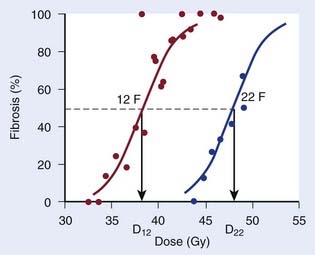
Repair at the cellular level has traditionally been seen as a manifestation of sublethal damage repair. At the tissue (or clinical) level, the term recovery is preferred by some authors as a more phenomenologic description of the recovery from damage observed when splitting the same physical dose into fractions, without assuming a specific cellular or molecular mechanism behind this effect. The clinical manifestation of recovery is the decreased biologic effect resulting from delivering a constant physical absorbed dose with decreasing dose per fraction. Fig. 3-1 shows dose-response curves for the incidence of moderate and severe (G2+) subcutaneous fibrosis. Note that the doses are estimated at the relevant reference depth for subcutaneous fibrosis10; in other words, they are not identical to the prescribed dose to the target delivered in 12 or 22 F. The dose, D12, corresponding to a 50% incidence of G2+ subcutaneous fibrosis is lower than the dose, D22, that would produce the same incidence in the 22 F group. The two doses are related by a mathematic relationship—the LQ model. This fractionation effect has been observed in countless studies, perhaps most clearly in clinical studies in which a larger dose per fraction has been introduced without any reduction in total dose. The classical example is the breast radiotherapy study by Montague11 in which 35 to 40 Gy was delivered across 4 weeks, giving 5 F per week in 88 patients and 3 F per week without a total dose reduction in 30 patients. The incidence of late complication was much higher in the large dose-per-fraction group. More support comes from studies in which the dose per fraction has been increased, but although a reduction of total dose was implemented, this later turned out to be insufficient. This occurred, for example, in studies12,13 using the nominal standard dose formula created by Ellis14 as a guide for reducing the dose, which effectively led to an over-dosage of late normal-tissue endpoints.
In addition to the magnitude of recovery, the kinetics of recovery is important for biologic effect. A dramatic illustration of this is the study by Nguyen et al.15 in which 39 patients received rapid hyperfractionated radiotherapy: 6 to 8 F of 0.9 Gy per day with a 2-hour interval between fractions were delivered five days a week for a total dose of 66 to 72 Gy. Radiotherapy was delivered in two series of 33 to 36 Gy separated by a 2- to 4-week rest interval. If the 2-hour interval had been sufficient for complete or near-complete recovery, this dose should have been relatively well-tolerated. Instead, after a minimum follow-up of 2 years, 70% of patients experienced late complications, and in 54% of cases these reactions were considered severe, causing death in 13% of patients.
Repopulation is clinically reflected in the influence of overall treatment time on local control of at least some tumor types (in which it is often called accelerated proliferation) and on the incidence of some early normal tissue effects. This phenomenon is often referred to as the time factor, a term that has the advantage of referring to a clinically observable effect rather than to an underlying hypothetical cellular mechanism. Several studies tried to estimate the tumor time factor by comparing patients who completed therapy in the planned overall time versus patients who had protracted overall time resulting from unplanned treatment interruptions.16 A strong case can be made, however, that patients with and without unplanned interruptions are not likely to present with comparable tumor and patient characteristics.17 Much stronger evidence has subsequently been obtained from randomized controlled trials, at least for some tumor types.
Redistribution of the number of cells in various phases of the cell cycle is observed after irradiation of an asynchronous cell population caused by varying radiosensitivity in these phases. There is no directly observable clinical parallel to redistribution. It is interesting to note that the European Organisation for Research and Treatment of Cancer (EORTC) 22791 trial by Horiot et al.18 used two fractions per day in an attempt to “catch” the more rapidly proliferating tumor cells that were hypothesized to have progressed into a more sensitive phase of the cell cycle at the time of the second daily fraction.19 When this trial was completed, the data were widely interpreted in terms of a differential sensitivity to dose per fraction (i.e., as a manifestation of differences in repair or recovery capacity) as predicted by the LQ model. Redistribution is also of great interest in combining drugs with radiation and many cytotoxic drugs such as cisplatin, 5-fluorouracil (5-FU), and gemcitabine require cell-cycle progression to act as radiosensitizers.20 Carefully timed administration of drugs and radiation has been proposed in an attempt to synchronize surviving tumor cell populations and then irradiate them in a sensitive phase of the cycle—an idea that so far has not worked convincingly in clinical trials, most likely because human cell populations in vivo are so heterogeneous in their cell kinetics parameters that synchrony is quickly lost in a population of patients.
Reoxygenation refers to the empirical observation that hypoxic regions in tumors may improve their oxygenation during fractionated radiotherapy. Traditionally, this has been viewed as a consequence of preferential killing by radiation of well-oxygenated cells that in turn leads to a lower metabolic consumption of oxygen, which again leads to improved oxygenation of the predominantly hypoxic cells surviving a dose fraction. The kinetics of reoxygenation is not well-studied in humans. However, a wide tumor-to-tumor variability in reoxygenation has been detected in human tumors by means of positron emission tomography scan using hypoxia-sensitive tracers.21 Because many human tumors, in contrast to most normal tissues, contain hypoxic cell populations, reoxygenation provides further rationale for fractionated radiation therapy. Advances in hypoxia-related cancer research suggest that this rather simple model of hypoxia and its modification during fractionated radiotherapy is an over-simplification. Hypoxia is now seen as an integral aspect of malignant progression and as an active biologic process rather than the passive push of cells into oxygen deprivation.22 Hypoxia-mediated radioresistance is also emerging as an actively controlled phenomenon, with the hypoxia-inducible factor–1α as a key player, and not just a direct consequence of the physicochemical absence of molecular oxygen.23–25 From a clinical radiation research perspective, many strategies have been devised to modify tumor hypoxia, including treatment in hyperbaric oxygen, administration of electron-affinic oxygen mimetic drugs such as nitroimidazoles,26 or hypoxic cytotoxins such as tirapazamine.27 These have been plagued by logistic difficulties and unexpected toxicities, but more discouragingly have yielded modest improvements in tumor control.28
The Linear-Quadratic Model
Mechanistic Background
The LQ model originated from work by Lea and Catcheside in Cambridge around the time of World War II.28a In a series of published studies, they investigated the influence of dose and dose rate on chromosome damage in cells. Lea and colleagues developed a framework for interpreting their experimental data in terms of inactivation of discrete targets.28b They hypothesized that inactivation could result from single or double “hits” and fitted an expression of the form α · D + β · D2 to experimental data on the number of chromatid exchanges per cell as a function of dose. Curiously, they used the notations α and β for the two coefficients in their “linear-quadratic” equation.28c Numerous investigators derived LQ bioeffect relationship under various assumptions; for example, Kellerer and Rossi29 published an elaborate theory of dual radiation action in 1972. However, it was the 1976 paper by Douglas and Fowler,30 in which they used the LQ model to fit data on skin reactions after fractionated radiotherapy, that stimulated the modern interest in the LQ model. The full effect plot devised by Douglas and Fowler facilitated the analysis of isoeffect data for any sign or symptom of radiation therapy without the need to know the underlying target cell survival curve. At the same time, the Fe plot provided a simple graphic test of the fit of the LQ model to the data. A few years later, Thames and colleagues31 realized that the numeric value of the ratio of the two model parameters, α/β, differed between early and late effects of radiation therapy, with values for early effects typically ranging from 8 to 12 Gy and for late effects between 1 and 5 Gy. Thames and colleagues hypothesized that the difference in α/β reflected differences in the curvature of the dose-survival curve of the putative target cells. The compelling link between the LQ model and the target cell hypothesis remained strong for many years, but this has come under increasing pressure recently.
Beyond the Target Cell Hypothesis
Advances in molecular pathology have considerably improved our understanding of radiation-induced pathologic conditions of late normal tissue effects in particular.32 It has become clear that many late effects result from a powerful, sustained wound healing response at the tissue level rather than simple parenchymal cell loss. The biology of this “fibrogenic-atrophic” radiation response pathway has been unraveled in quite some detail during the preceding decade or so. A key switch in this response is the activation of the multifunctional, strongly profibrotic cytokine transforming growth factor (TGF)-β. Ionizing radiation is one of the few exogenous factors that can activate TGF-β directly. Thus the target cell hypothesis may not explain the main pathogenic pathways for late effects. This is in contrast to the radiation-induced pathologic conditions of early effects that typically occur in tissues with a hierarchical proliferative organization and depend on the relative depletion of the stem cell pool.33 In the present context, this puts a question mark over the traditional explanation of the difference in α/β ratio between early and late effects, namely that this reflects differences in the shape of the (in vivo) cellular dose-survival curve for the putative target cells giving rise to the two types of radiation effects. At the time of writing, it is not clear what part of the TGF-β pathways determines the relatively high fractionation sensitivity of late effects. Suffice it to say that an overwhelming body of clinical and experimental data show that the dose adjustment required for maintaining a constant level of side effects when dose per fraction is changed is much larger for late than for early endpoints. This “postmodern” view of the LQ model simply acknowledges the empirical success of the model in estimating biologically equivalent doses when changing dose-fractionation—at least within a limited dose range—but does not presume any deeper mechanistic validity of the mathematic form of this model.
Pragmatic Derivation—Correction for Dose per Fraction
Other functional forms could work as well, but this expression is as simple as it gets. Now we are ready to derive the isoeffect formula, referred to as the Withers formula. Two dose fractionation schedules, delivering a dose D1 in dose per fraction d1, produces the same biologic effect as a dose D2 delivered in dose per fraction d2, if and only if:
This follows from the assumption that f is a strictly increasing function. We assume that the overall treatment time is identical in the two schedules and that redistribution and reoxygenation can be ignored. Equation 2 can easily be rearranged to yield:
Dividing by β on both sides of the equation yields:
Finally, we isolate D1 on the left-hand side:
which is the so-called Withers formula.34 Note that there is only one parameter in this formula that needs to be estimated from clinical or experimental data: the α/β ratio. This formula describes the relationship between the two isoeffective dose in Fig. 5-1; or, alternatively, if we observe the shift in the dose-response curves, we can calculate the α/β ratio for the endpoint in question, subcutaneous fibrosis (in turns out to be α/β = 1.8 Gy10). More precise estimates can be obtained using statistical techniques and these also allow estimation of the uncertainty of the α/β (as well as other model parameters) and allow correction for the latent period and censoring in patients who were alive and well at the last follow-up.35,36 In other words, it is not necessary to know the separate values of α and β to estimate the biologically equivalent dose when changing from one fraction size to another. Up-to-date compilations of α/β values for experimental37 and clinical38 normal-tissue and tumor endpoints have been published recently.
For an endpoint with a known α/β ratio, Equation 3 can be applied to convert an arbitrary dose, D, delivered with dose per fraction, d, into an equivalent dose in 2-Gy fractions, (EQD2).38 This quantity is equivalent to the normalized total dose introduced by Withers et al.34:
A simple numeric example follows: A simultaneous integrated boost plan is being considered for a patient with HNSCC. The plan will deliver 66 Gy in 22 F to the gross tumor volume. Assuming that α/β = 10 Gy for HNSCC, what is the equivalent dose in 2-Gy fractions, EQD2? Inserting the known values in Equation 4, we get:
Recovery Kinetics
Split-dose recovery was discovered in cell lines in vitro by Elkind and Sutton39 in 1960. By varying the interval between two fractions (“splitting” the same physical dose in two), Elkind and Sutton were able to show how the two fractions had the same biologic effect as a single dose of the same size if the interval between fractions was very short, and how this effect asymptotically approached a certain minimum effect as the interval became very long. The same effect can be seen in clinical studies when the interval between fractions is varied, and this is also an important component in explaining the dose-rate effect in continuous irradiations. Mathematically, the effect of protracting therapy (i.e., delivering each dose fraction over longer and longer time) can be described by introducing the Lea-Catcheside factor (g), which can be seen as a factor modifying the effective fraction size:
Under fairly simple assumptions, the g-function can be expressed in analytic form for many of the situations arising in clinical radiation oncology such as continuous irradiation or multiple fractions per day (MFD) with incomplete repair between fractions (see, for example, Joiner and Bentzen37).
Correction for Overall Treatment Time
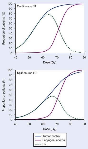
Empirically, the biologic effect of a given total dose delivered in a fixed number of fractions decreases with increasing overall treatment time (i.e., with increasing time between the first and last dose fraction). In case of tumor control, this effect is often referred to as the tumor time factor, and it is often interpreted as the result of tumor clonogen (cancer stem cell) proliferation in this time interval. Fig. 3-2 summarizes data from the Danish Head and Neck Cancer collaborative group (DAHANCA) comparing the outcome of fractionated radiotherapy delivered with 2-Gy fractions over 6 weeks and 10 weeks.40 With longer overall treatment time, the tumor dose-control curve shifted to the right; in other words, an increased dose was required to maintain the same level of tumor control. In contrast, the dose-response curve for laryngeal edema did not change. This caused a narrowing of the therapeutic window. Assuming that laryngeal edema and local failure are statistically independent,41 the probability of uncomplicated cure (P+) becomes TCPx (1 − normal tissue complication probability [NTCP]). The maximum value of P+ dropped from 78% for continuous course to 47% for split-course radiation therapy.
In other words, if total dose D2 is delivered in T2 days and T2 is greater than T1, we will subtract a (positive) dose from the estimated equivalent dose, reflecting the fact that biologic effect is lost because of the prolonged treatment time. It is assumed that both T1 and T2 are sufficiently long for accelerated proliferation to occur at a constant rate. As this formula is likely to be used in the comparison of two fractionation schedules, the arbitrary choice of the length of the reference schedule (T1) will cancel out.
The majority of empirical Dprolif estimates are derived from HNSCC data, in which this parameter consistently across a large number of studies38,42 comes out at approximately 0.65 Gy/day. This means that if a schedule is prolonged by, for example, 5 days, the estimated decrease in the EQD2 is 5 days × 0.65 Gy/day = 3.25 Gy. Mechanistically, the cellular proliferative response to a cytotoxic insult is a complex phenomenon,33,43,44 but this simple linear correction is likely to be a good approximation over a narrow range of treatment times, in the order of 1 to 2 weeks perhaps for a 6- or 7-week schedule. The numeric value of Dprolif cited previously is estimated toward the end of treatment schedules with an overall treatment time of some 5 to 7 weeks. Proliferation before the start of radiotherapy corresponds to a much lower dose per day. This phenomenon is called accelerated proliferation (or accelerated repopulation).
When does accelerated proliferation start? In their classic paper from 1988, Withers et al.45 proposed that isoeffect doses for local control of HNSCC remained largely constant up until approximately 4 weeks of overall treatment time, after which accelerated proliferation would kick in and the dose lost per day because of proliferation would be approximately 0.6 to 0.7 Gy/day. The appearance of this biphasic relationship, dubbed the dog-leg, depended on the exact assumptions of the modeling performed by Withers et al. to pool data from multiple studies on the same graph, and some authors—including the present one—argued that these assumptions were unrealistic46 and that the data could in reality not discriminate between the dog-leg shape and a straight line all the way down to very short schedules. A specific weakness of the available data was an absence of schedules treating in less than 4 weeks.
The continuous, hyperfractionated, accelerated radiotherapy (CHART) trial is very interesting in this context, as the experimental CHART arm finished radiotherapy in only 12 days. This provides a sensitive test for the existence of the “kink” on the dog-leg graph (Fig. 3-3). As CHART employed 1.5-Gy fractions, we use Equation 4 with an assumed α/β of 10 Gy (this parameter should ideally be estimated from the data as well) to calculate the EQD2 of the CHART arm: 51.75 Gy. From the reported hazard ratio (HR) derived from the 918 patients in the trial, we can calculate the apparent dose in 2-Gy fractions that would be isoeffective with 66 Gy in 45 days: the result is 51.3 Gy with 95% confidence limits 49.3 Gy and 53.3 Gy, plotted in Fig. 3-3. This is considerably higher than the 44.6 Gy estimated from back-extrapolating the 66 Gy by 0.65 Gy/day all the way down to 12 days’ overall time. In other words, delivering dose in just 12 days is not nearly as effective as one would estimate if the dose recovered per day was constant all the way down to 12 days.*
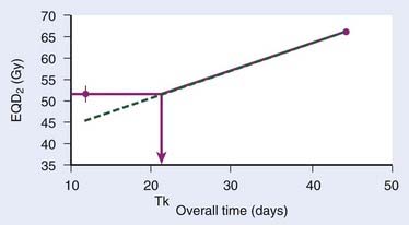
Thus, Withers turned out to be right: our current best estimates of the radiobiologic parameters for accelerated repopulation are almost exactly as derived in the 1988 paper. This has huge implications for how far accelerated fractionation schedules can be pushed. It is difficult from the available data to decide whether dose recovery with extended treatment time is truly a biphasic relationship or whether there are more phases. What is clear, however, is that a constant rate of proliferation corresponding to a recovered dose of Dprolif = 0.6-0.7 Gy/day cannot be back-extrapolated all the way down to schedules of 1 or 2 weeks’ duration. The standard way to incorporate this phenomenon in the modeling of the overall time effect is to assume Dprolif = 0 Gy/day up until a defined kick-off time (Tk) and then assume a constant Dprolif thereafter (see Fig. 3-3). In practice, this means that if T1 or T2 (or both) is shorter than Tk then this (or these) times are set equal to Tk when entered into equation 6.
Alternative Formulations of the LQ Model
A couple of mathematically equivalent formulations of the LQ model have been used as alternatives to the EQD2 formula. Among these, only the biologically effective dose (BED) formula has found any wider use.47

Stay updated, free articles. Join our Telegram channel

Full access? Get Clinical Tree


