Abbreviations
- ARR Absolute risk reduction
- CI Confidence interval
- CV Coefficient of variation
- EBM Evidence-based medicine
- ER Event rate
- NiH Negativity in health
- NNT Number needed to treat
- PiD Positivity in disease
- QALY Quality-adjusted life year
- RCT Randomized controlled trial
- ROC Receiver-operating characteristic
- RRR Relative risk reduction
- USPSTF U.S. Preventive Services Task Force
Evidence-Based Endocrinology and Clinical Epidemiology: Introduction
The individual practitioner faces a multiplicity of potential diagnoses, limitations in diagnostic capacity, subclinical disease identified by tests rather than by clinical manifestations, and rapid changes in scientific knowledge. The paradigm of clinical decision-making based on the assumption that all that is needed to guide clinical practice is personal experience (however unsystematic), understanding of pathophysiology, and thorough training plus common sense is insufficient to address these challenges. Moreover, the integration of relevant research findings into clinical practice has been haphazard; the lag time between development of scientific knowledge and introduction into practice can be many years, and there is marked variation in practice. A systematic approach based on principles of clinical epidemiology can help address some of these issues. This quantitative approach has formed the primary, albeit not the only, basis of the evidence-based medicine movement. This movement posits that understanding certain rules of evidence is necessary to interpret the literature correctly and that physicians who practice based on the above understanding will provide superior care. This chapter will summarize some of the principles of clinical epidemiology and evidence-based endocrinology and some of their limitations.
Clinical Epidemiology
Clinical epidemiology consists of the application of epidemiologic principles and methods to problems encountered in clinical medicine. Clinical epidemiology emphasizes a quantitative approach and is therefore concerned with counts of clinical events. Its applications are paramount (1) in diagnostic testing and how the results modify the probability of a particular disorder being present and (2) in treatment decisions in which the potential benefits and harms must be addressed. The techniques of clinical epidemiology have become increasingly important as practitioners confront the complexity of contemporary medical practice.
Diagnostic Testing: Test Characteristics
The appropriate choice and interpretation of diagnostic tests, whether biochemical assays, radiologic procedures, or clinical findings, have always been essential to the clinical practice of endocrinology. These tests, when introduced in the medical literature, are accompanied by varying degrees of validation. The clinician’s assessment of the utility of tests, now even more important with the emphasis on cost-effectiveness, can be improved by knowledge of test EBM principles. We review some of these concepts as they apply to diagnosis and management of endocrine disorders, including the topics of test characteristics such as sensitivity and specificity, receiver-operating characteristic (ROC) curves, likelihood ratios, predictive values, and diagnostic accuracy.
The evaluation of endocrine function begins with a clinical question. The more vague the question, the more difficult it is to obtain a clear answer. Part of this step involves a clinical judgment about the likelihood of the disease prior to obtaining a test and its results. This pretest probability is combined with the performance characteristics of the test and its use (sensitivity and specificity, ROC curves, likelihood ratios, predictive values, and diagnostic accuracy) in order for proper interpretation. Variation is inherent in biological systems. Therefore, diagnostic tests must take into account not only variability of the tests themselves and how they are performed but also variability in the populations in whom the tests were developed, both with the disease and without the disease. Key aspects in the analysis of a test include reproducibility (precision) and accuracy. Reproducibility describes how close the test comes to producing the same results every time and depends on such factors as intraobserver and interobserver variability (as in the assessment of a physical finding or x-ray) and, in the case of biochemical tests, characteristics such as intra-assay and interassay coefficients of variation (CVs). Although studies utilizing radioimmunoassays and other assays routinely report intra-assay and interassay CVs, few papers publish multiple results performed on the same patient (intraindividual variation). There have also been relatively few studies on the reliability of measurements (ie, the degree of intraindividual variation). One study found that the minimum number of replicate measurements necessary to achieve satisfactory reliability of the mean of basal levels was 3 for plasma cortisol and 18 for salivary cortisol. Responses to dynamic tests required fewer replicates to achieve the same reliability (one to two samples).
Reproducibility depends on the conditions under which the test is performed. Clinicians must be aware of the distinction between efficacy and effectiveness when translating published results into practice. As applied to diagnostic testing, efficacy refers to the degree to which the test has been shown scientifically to accomplish the desired outcome. In contrast, effectiveness refers to the degree to which the test achieves this outcome in actual clinical practice. Most large studies have been performed in research venues and thus are efficacy studies, whereas the effectiveness of most tests in practice has not been extensively evaluated. In comparing one’s own results with a published report or laboratory normal range, it is important to take into account those conditions (eg, test performed in a hospital vs a physician’s office).
Accuracy describes how close the test comes to producing results that are a true measure of the phenomenon of interest; systematic bias of a highly reproducible test may produce the same incorrect result every time. Like reproducibility, accuracy depends on the conditions under which the test is performed; accuracy in the clinical practice setting may differ from that in the experimental setting where many extraneous influences are controlled.
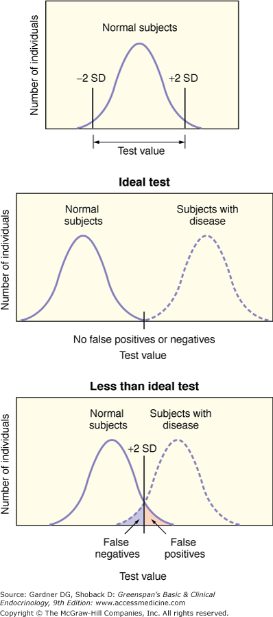
When interpreting a test, the result is usually compared to a normal range. Frequently, the normal range is developed by using a reference population assumed (or preferably shown) to be disease free. For example, when designing a test to be used in the diagnosis of Cushing syndrome, the reference group should be made up of individuals who have clinical features suggestive of Cushing syndrome but who in fact do not have the disorder. However, reference groups may be made up of individuals who are readily accessible and not more appropriate comparisons. It is also important to note that in establishing a normal range based on a Gaussian or normal distribution, encompassing the mean ± two standard deviations, 5% of disease-free individuals have a result outside the limits of normal. (It is important to note that the definition of normal based on a Gaussian distribution of values is only one of a number of definitions of normal. Some others include the one most representative or most common in a class, the one most suited to survival, and the one that carries no penalty [ie, no risk].) Figure 3–1 illustrates a normal range and a range in a population with disease. A result outside normal limits is not equivalent to disease. Moreover, values within the normal range do not necessarily exclude disease. Values in the population of individuals with disease are determined separately, and the overlap with the normal range is assessed.
Figure 3–1
Defining a normal range and diagnostic testing. The top panel shows the Gaussian (normal) distribution of test values in a population of individuals. The middle panel illustrates two such curves that describe the findings in an ideal test. In this case, there is no overlap in the results between normal subjects and subjects with disease (ie, there are no false-positive results and no false-negative results). The bottom panel illustrates the results for a less-than-ideal test. Normal subjects with test values above the given threshold have abnormal results (ie, false-positive results), whereas some subjects with disease have test values below that threshold (ie, normal or false-negative results).
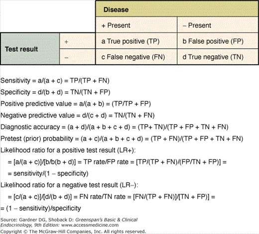
Ideally, a diagnostic test has no overlap between the results of individuals with the disease and those without the disease. The reality, however, is different. Test characteristics that describe this overlap are sensitivity and specificity, and they are typically illustrated in a 2 × 2 table. As shown in Figure 3–2, sensitivity and specificity are collectively known as operating characteristics. Sensitivity refers to the ability to identify correctly individuals with a disease. The sensitivity of a sign or symptom (or diagnostic test) is the proportion of patients with disease who has a positive test result, sign, or symptom. In contrast, specificity refers to the ability to identify correctly individuals without a disease. The specificity of a test is the proportion of healthy patients who have a negative test result or who lack that sign or symptom.
Thus, the sensitivity of a test equals the number of individuals with disease who have a positive test (true positive [TP] divided by the number of individuals with disease (true positives plus false negatives [FN]), whereas specificity equals the number of individuals without the disease who have a negative test (true negatives) divided by the number of individuals without disease (true negatives plus false positives [FP]). Sensitivity is sometimes termed PiD or positivity in disease, and specificity is sometimes termed NiH or negativity in health. In theory, sensitivity and specificity are characteristics of the test itself and not of the patients on whom the test is applied. However, this may not be correct in practice. The sensitivity of a test may be affected by the stage or severity of the disease. The specificity of a test may depend on the characteristics of the reference population. The nature of the groups used to establish the cut-points that differentiate normal from abnormal must be appropriate and should be specified in any report of a diagnostic test. The value chosen for a cutoff point also affects the sensitivity and specificity. To assist the clinician in assessing a report on a diagnostic test, a series of questions has been proposed (Table 3–1).
| Question #1 | Is the study population described well enough? |
| Question #2 | Does the spectrum of illness in the study population differ from that of my patients (eg, spectrum bias)? |
| Question #3 | Was a positive result on the index test a criterion for referral to have the gold standard test? |
| Question #4 | Was there blinding of those who interpreted the index test and those who interpreted the gold standard test (eg, test review bias)? |
| Question #5 | Was the gold standard test an adequate measure of the true state of the patient? |
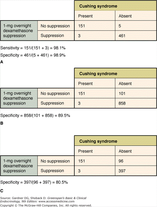
The overnight dexamethasone suppression test is commonly used as a screening test in the diagnosis of Cushing syndrome, and its use illustrates some of the issues in diagnostic testing. As shown in Figure 3–3, combining the results of a number of studies indicates a sensitivity of 98.1% and specificity of 98.9%. However, the individual studies varied, with sensitivities ranging from 83% to 100% and specificities from 77% to 100%. Moreover, the studies used different cortisol assays, doses of dexamethasone, and criteria for a positive test. Caution must be exercised in drawing conclusions from the combining of such data. In order to apply the sensitivity and specificity of a test derived from one study sample to a different population, the test cannot deviate from methods used (eg, dose of dexamethasone, type of cortisol assay, timing of dexamethasone administration, and cortisol assay) when the optimal cutoff was determined, and the sample studied must be similar to the new population to be tested. To meet this latter prerequisite, the sample studied must account for variability of diseased individuals. This requires that subjects with disease be defined using the best available gold standard (independent of the test in question) and include a broad enough cross-section of those with disease (eg, mild versus severe disease, different etiologies of disease, as well as age, sex, and race) to establish a reliable range of measurements. The characteristics of the reference sample of subjects without the disease are equally important. Although the 1-mg overnight dexamethasone suppression test is still believed to have excellent, albeit less than 100% sensitivity, it has serious problems with specificity, and false-positive results have been described with a variety of drugs as well as medical, surgical, and psychiatric conditions.
Figure 3–3
Diagnosis of Cushing syndrome with the 1-mg overnight dexamethasone suppression test: test characteristics with normal controls (Panel A); all controls (Panel B); and “obese” and “other” controls (Panel C). These data show how the specificity of the test is affected by the types of control subjects.
(Reproduced with permission from Crapo L. Cushing’s syndrome: a review of diagnostic tests. Metabolism. 1979;28:955.)
One additional method of reporting the performance of a test is diagnostic accuracy. This can also be derived from the 2 × 2 table. Diagnostic accuracy is defined as the ability of a test to identify correctly those with the disease and those without the disease:
From Crapo composite data on the 1-mg overnight dexamethasone suppression test, the diagnostic accuracy is calculated as 98.7%. In addition to the characteristics of the study subjects, the number of subjects included in the sample is also critical to assess the accuracy of the test. Each operating characteristic determined in a study should be accompanied by a confidence interval (CI)—a range of values calculated from sample size and standard error which expresses a degree of confidence (usually 90%, 95%, or 99%) that the unknown true sensitivity or specificity lies in that interval. CIs are a measure of the precision of an estimate. The range of a CI depends on two factors: (1) the number of observations; and (2) the spread in the data (commonly measured as a standard deviation). The fewer the number of observations, the larger the range of the CI, and the greater the standard deviation of the data, the larger the range of the CI.
In addition to the limitations on the operating characteristics based on the samples from which the data are derived, sensitivity and specificity are not independent of each other. They vary with the cutoff level chosen to represent positive and negative test results. In general, as sensitivity increases, specificity decreases and as specificity increases, sensitivity decreases. This phenomenon is depicted graphically in an ROC curve.
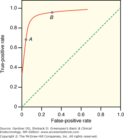
An ROC curve graphically illustrates the trade-off between the false-negative and false-positive rates for different cutoff points of a diagnostic test. In an ROC curve, the true-positive rate (sensitivity) is plotted on the vertical axis and the false-positive rate (1−specificity) is plotted on the horizontal axis for different cutoff points for the test. The dotted diagonal line in Figure 3–4 corresponds to a test that is positive or negative just by chance (ie, the true-positive rate equals the false-positive rate). Such a test provides no useful information. Ideally, a test would provide results that could be plotted on one point in the top left corner—100% true-positive rate and 100% true-negative rate. The closer an ROC curve is to the upper left-hand corner of the graph, the more accurate it is, because the true-positive rate is 1 and the false-positive rate is 0. As the criterion for a positive test becomes more stringent, the point on the curve corresponding to sensitivity and specificity (point A) moves down and to the left (lower sensitivity, higher specificity); if less evidence is required for a positive test, the point on the curve corresponding to sensitivity and specificity (point B) moves up and to the right (higher sensitivity, lower specificity). Analysis of the area between the actual results and the straight line indicates how good the test is. The greater the area under the curve, the better the test.
Figure 3–4
Receiver-operating characteristic (ROC) curve. In an ROC curve, the true-positive rate (sensitivity) is plotted on the vertical axis, and the false-positive rate (1 − specificity) is plotted on the horizontal axis for different cutoff points for the test. The dotted diagonal line corresponds to a test that is positive or negative just by chance (ie, the true-positive rate equals the false-positive rate). The closer an ROC curve is to the upper left-hand corner of the graph, the more accurate it is, because the true-positive rate is 1 and the false-positive rate is 0. As the criterion for a positive test becomes more stringent, the point on the curve corresponding to sensitivity and specificity (point A) moves down and to the left (lower sensitivity, higher specificity); if less evidence is required for a positive test, the point on the curve corresponding to sensitivity and specificity (point B) moves up and to the right (higher sensitivity, lower specificity). Analysis of the area between the actual results and the straight line indicates how good the test is. The greater the area under the curve, the better the test.
Depending on the purpose of the test, the curves may be used to decide an optimal cutoff level for a single test. For example, with a screening test, high sensitivity is typically desired, and the trade-off is lower specificity. The cutoff point may also be chosen depending on health costs (morbidity and mortality associated with an error in diagnosis), financial costs, or need for maximal information (the operating position giving the greatest increase in posttest probability).
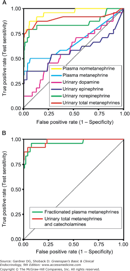
ROC curves may also be used to compare two or more tests by comparing the areas under the curves, which represent the inherent accuracy of each test. An example of the comparison of the performance of different tests for the diagnosis of pheochromocytoma is given in Figure 3–5. It is important to remember, however, that ROC curves are only as good as the operating characteristics from which they are generated.
Figure 3–5
Receiver-operating characteristic (ROC) curves for diagnostic tests for pheochromocytoma. Receiver-operating characteristic (ROC) curve. In an ROC curve, the true-positive rate (sensitivity) is plotted on the vertical axis, and the false-positive rate (1 – specificity) is plotted on the horizontal axis for different cutoff points for the test. A diagonal line drawn for the points where true positive rate = false positive rate corresponds to a test that is positive or negative just by chance. The closer an ROC curve is to the upper left-hand corner of the graph, the more accurate it is, because the true-positive rate is 1 and the false positive rate is 0. As the criterion for a positive test becomes more stringent, the point on the curve corresponding to sensitivity and specificity moves down and to the left (lower sensitivity, higher specificity); if less evidence is required for a positive test, the point on the curve corresponding to sensitivity and specificity moves up and to the right (higher sensitivity, lower specificity). Analysis of the area between the actual results and the line representing chance alone indicates how good the test is. The greater the area under the curve, the better the test. The area under the curve from plasma-free metanephrines exceeds that of other tests indicating that it is more accurate overall.
Finally, determining cost-effective diagnostic strategies requires careful evaluation not only of a test in isolation, but also in the context of the other information available and the likelihood of disease. This is the essence of Bayesian models of decision-making. In this model, the physician updates his or her belief in a hypothesis with each new item of information, with different weights given to the new information depending on its operating characteristics. Consideration must be given to the question of the value added by a test or procedure. This can be assessed with ROC curves and statistical models.
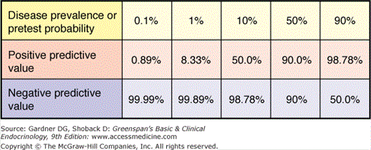
Sensitivity and specificity are important test characteristics, yet the clinician wants to know how to interpret a test result. Predictive values help in this regard. As shown in Figure 3–6, the positive predictive value is the proportion of patients with a positive test who actually have the disease. Similarly, the negative predictive value is the proportion of those with a negative test who do not have the disease. Because each of these values are calculated using results from both individuals with and without the disease in question, the prevalence of the disease has a great impact on the values. For any given sensitivity and specificity, the lower the prevalence of disease (or the lower the pretest probability), the more false-positive results there are (Figure 3–6).
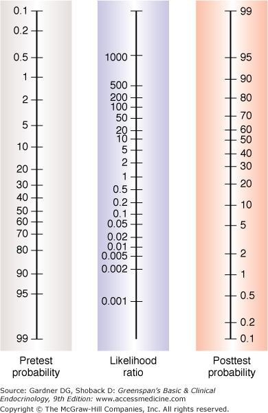
The likelihood ratio, which is derived from sensitivity and specificity, is an expression of the odds that a sign, symptom, or test result is expected in a patient with a given disease as opposed to one without the disease. Two forms of the likelihood ratio exist, the likelihood ratio for a positive finding and the likelihood ratio for a negative finding. Calculations are shown in Figure 3–2. Likelihood ratios offer some advantages over sensitivity and specificity. They are the most useful in calculating posttest probabilities given prevalence (a probability) and likelihood ratios. A convenient nomogram for this has been published (Figure 3–7).
An Approach to Diagnosis in Practice
In approaching a case, the clinician makes a series of inferences about the nature of a patient’s condition and proceeds toward a working diagnosis along with some alternatives—generation of a differential diagnosis. Although one could create a listing of all possible causes of the patient’s complaint (ie, a possibilistic differential diagnosis), experienced clinicians generate a differential diagnosis that is a combination of probabilistic (ie, considering first those disorders that are more likely), prognostic (ie, considering first those disorders that are more serious if missed), and pragmatic (ie, considering first those disorders that are most responsive to treatment). The clinician then refines the diagnostic hypotheses, sometimes using clues from the history and physical examination and often with the use of laboratory or radiologic tests. In so doing, the clinician tries to reduce the inherent uncertainty so that the most appropriate course of treatment can be prescribed.
The first step in this process is to understand the concept of probability. A probability is an expression of likelihood and thus represents an opinion of the relative frequency with which an event is likely to occur. In the case of diagnosis, probability is a numerical expression of the clinician’s uncertainty about a diagnosis; expressing a clinical opinion in subjective terms such as likely and possible is fraught with imprecision and misunderstanding. Certainty that a disease is present is assigned a probability of one, certainty that a disease is not present is assigned a probability of zero, and a clinician’s opinion of the disease being present or absent usually falls somewhere in between. Of course, probabilities are derived from different data sources that vary in their reliability and application to a given patient, such as the clinician’s experience (remembered cases), research studies, and population-based epidemiologic studies. Therefore, some degree of uncertainty is inherent in a given probability, and the confidence with which one can rely on a given probability depends to a large extent on the data underlying it.
The diagnostic approach to minimizing uncertainty requires four steps. First, the clinician starts with an estimate of probability based on initial clinical impressions. This starting point is dubbed the pretest or a priori probability and is a number between zero and one that expresses the likelihood of disease. For example, a clinician who sees a large population of patients with diabetes mellitus may think that a 55-year-old patient with polyuria, polydipsia, weight loss, and fatigue has a probability of 0.70 of having diabetes mellitus (ie, if there were 100 such individuals, 70 would have diabetes).
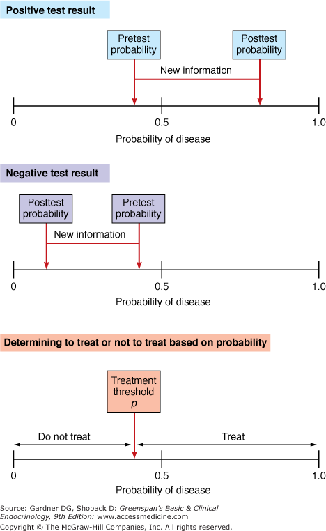
Second, the clinician determines the threshold probability for treatment. The treatment threshold probability is defined as the probability of disease at which one is indifferent between giving treatment and withholding treatment. Establishing a treatment threshold probability takes into account the costs (not just in the monetary sense) and benefits of treating or not treating. Because probability is predicated on the lack of certainty about the presence or absence of disease, it is inevitable that some patients who are not diseased receive treatment and others who are diseased do not receive treatment. Third, if the pretest probability is greater than the threshold probability, the clinician chooses to treat; if it is less than the threshold probability, the clinician opts not to treat. If the clinician is not comfortable enough about the presence or absence of disease, he or she may choose to order further tests with the objective of getting closer to certainty. The fourth step involves taking information gained from the test and using it to update the pretest probability. The updated, or posttest, probability can also serve as a new pretest probability for the next step in hypothesis testing (Figure 3–8).
Figure 3–8
Adjusting probabilities with new information and treatment thresholds. The top panel shows a pretest probability of disease of approximately 0.4. With the new information provided by a test, the probability rose to approximately 0.7. The middle panel shows the same pretest probability, but a negative test result reduced the probability of disease to approximately 0.15. The treatment threshold probability is the probability above which one would treat. The actual threshold value depends on the morbidity and mortality of disease and the adverse effects (morbidity and mortality) of treatment.
