Chapter 3
Endoplasmic Reticulum- and Plasma-Membrane-Driven Calcium Oscillations
Arthur Sherman
Laboratory of Biological Modeling, NIDDK, National Institutes of Health, USA
3.1 Introduction
Calcium ( ) is of great importance throughout biology because it regulates many processes. In neuroendocrine cells, it plays a central role as the main trigger of hormone and peptide secretion. In the experimental literature, one often finds statements along the lines of “Agent X increases
  concentration (
 ), which increases secretion”. However, secretion is generally not controlled by a mere rise and fall of
  concentration, but rather by
  oscillations, and “Agent X” works by changing the pattern of those oscillations.
One of the key contributions of theorists has been to develop models that explain the mechanisms behind such oscillations and how they are regulated. Indeed, there are multiple mechanisms, so it is helpful to distinguish their origins and how they are regulated. In particular, we find oscillations that reflect variation in  influx and arise from ion channels at the plasma membrane (PM), as well as oscillations that reflect release from internal stores and arise from ion channels in the membrane of the endoplasmic reticulum (ER). A particularly interesting scenario, where the analytical power of models really shines, is when both mechanisms are present in the same cell and interact with each other.
Our objectives are limited. We will consider simplified examples that illustrate the basic principles rather than aim to model in detail any particular system. An understanding of these principles will provide good preparation to tackle particular problems in the future. Our focus is cellular; other chapters will address systems level models that involve multiple cell types and organs. We also limit ourselves to temporal phenomena, modeling cells as spatially homogeneous. This is often adequate, sometimes not. Mathematically, this means that we only need to deal with ordinary differential equations (a single independent variable, time), rather than partial differential equations (time plus one or more spatial dimensions.) We also treat only deterministic systems, which leaves out the sometimes important effects of noise, but allows us to make good use of dynamical systems tools, such as phase planes and bifurcation diagrams (BDs).
3.2 Calcium balance equations
3.2.1 Derivation
The fundamental physical principle needed to model calcium dynamics in cells is the conservation of mass, which is determined by flux across boundaries. In physics, flux is the rate of flow of some quantity per unit area (http://en.wikipedia.org/wiki/Flux). As we will be dealing with small round cells with a fixed boundary, it is convenient to multiply implicitly by the cell surface area, giving just quantity per time, symbolized by  . Our goal is to calculate the changes in the cytoplasmic or intracellular
  concentration,
  , denoted here more simply as
  , which means that we must divide by the cytosol volume to convert the rate of flux to the rate of change of concentration. The cytosol volume can be taken to be fixed, so that we can further simplify by absorbing the volume into the flux; we denote this scaled flux by
  .
.
Cells can often (but not always) be well approximated with two compartments: one for the cytosol and one for the ER, as shown in Figure 3.1. The cytosolic  ,
,  , then satisfies the equation
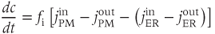
where we are using the volume-scaled fluxes.
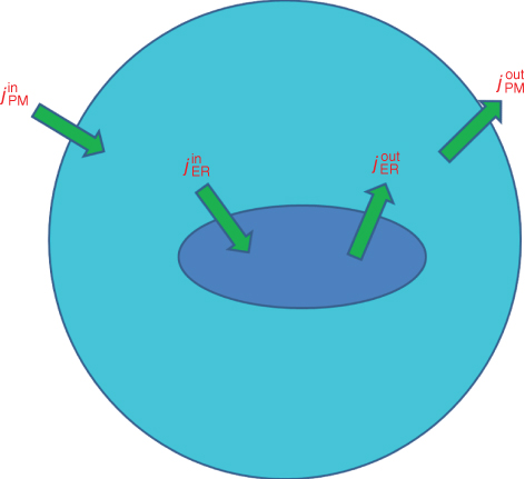
Figure 3.1 Calcium balance.  , influx through plasma membrane;
  , efflux through plasma membrane;
  , influx through ER membrane;
  , efflux through ER membrane.
The factor  accounts for the fact that most of the
  that enters a cell is buffered, that is, complexed with
  -binding proteins. Typically, only about 1% of the
  ions that enter remain free, which means that the rate of increase of the free
  concentration is only 1% of what it would be in the absence of buffering. This keeps the free concentration low and prevents runaway activation of the many reactions that are regulated by
  . This form of the equation is valid only because the buffering reactions are much faster than
  fluxes, so that it is safe to assume that free and bound
  are in the quasi-steady state. (A more complete derivation of this can be found in Sherman et al. (2002)).
The equation for ER  ,
,  , can be similarly written as
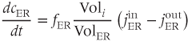
Note that the ER gets its own fraction of free  , which may differ from that in the cytosol. Also, because we absorbed the cytosolic volume into the fluxes, we have to multiply by the cytosolic-ER volume ratio to get the correct effect of the flux on
  . The ER volume is much smaller than that of the cytosol, so that the concentration change due to the flux will be much greater in the ER. However, the ER
  concentration is much greater, so the most typical case is small relative changes in the ER that result in large relative changes in the cytosol. We can make Equation (3.2) look much better, and reduce the number of parameters from 4 to 2, by multiplying the right-hand side by
  :
:
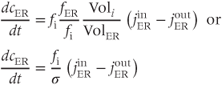
where

3.2.2 Applications
We will flesh out the  equations (3.1) and (3.3) and incorporate them into more complex models shortly, but pause here to show that even these simple equations can be used to draw nontrivial conclusions.
We choose the following expressions for the fluxes:


where PMCA is the “plasma-membrane calcium ATPase,” which pumps  out of the cell, and SERCA is the “sarco-endoplasmic reticulum calcium ATPase,” which pumps
  into the ER. We assume that flux out of the ER is a passive, diffusive leak. Equations (3.4) and (3.5) correspond to Equation (2.15), Chapter 2, this volume, for bulk cytosolic
  , except that the plasma-membrane calcium current is for the moment constant, not voltage dependent. In general, the pump expressions are not linear, but rather saturating Hill functions, but these are not needed for the moment. There may also be multiple plasma-membrane
  currents (e.g., L-type and T-type currents, as described in Chapter 2, Equations (2.6) and (2.7)), multiple ER
  channels (e.g., IP3 and Ryanodine receptors), and more than one
  efflux component (e.g., the
  –
– exchanger in addition to PMCA).
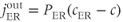
In Figure 3.2, the black curves show the effect of partial (50%) block of the SERCA pump, such as with thapsigargin, by cutting  in half. For simplicity, we assume that the block becomes fully effective instantaneously at
  min. Then,
  rises to a peak and then recovers to baseline. One often hears or reads something like “thapsigargin was used to increase
  ,” but the simulation shows that such an increase is only transient because the
  released from the ER to the cytosol is pumped out of the cell, leaving the ER depleted (in proportion to the inhibition of SERCA) but the cytosol at its original level once equilibrium is re-established. It is simple to show that the rise in
  must be transient: setting Equation (3.3) to steady state gives

and substituting this into Equation (3.1) and setting to the steady state implies that

Thus, the ER terms drop out of the  equation, and the steady-state value of
  depends only on the parameters of
  and
and  . We conclude that
  cannot be affected by the change in
  . The same would be true if we had emptied the ER by increasing efflux, which could correspond to the activation of IP3 or Ryanodine receptors. This is in general enough that it is worth stating as a theorem that holds independent of our choices for the fluxes:
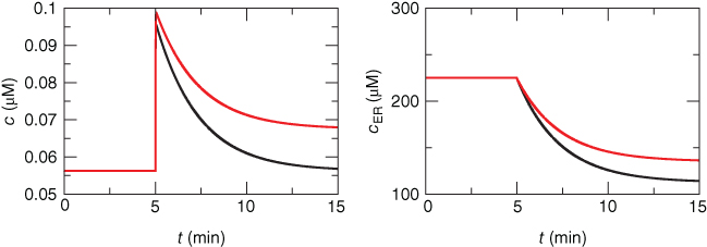
Figure 3.2 Illustration of the steady-state calcium theorem (Theorem 3.2.1) using the passive model, Equations (3.1) and (3.3), with fluxes as in Equations (3.4)–(3.7).  , cytosolic
  ;
;  , ER
, ER  . Parameters:
  M/pC;
M/pC;  pA,
pA,  pA (red), 0 (black);
  s
s ;
;  s
s , reduced to 0.2 s
 at
at  min;
min;  s
s ;
;  ;
;  .
.
A maintained change in  is illustrated by the red curve in Figure 3.2. In that simulation,
  is increased in magnitude at the same time that the PMCA is inhibited; this could correspond, for example, to a store-operated current (SOC) activated by the reduction in
  (Hogan et al., 2010). The combination of the two effects results in an increase in
  at the steady state. Conversely, if one observes a steady state increase in
  when SERCA is inhibited in an experiment, one can be sure that a plasma-membrane ion current was affected (though not necessarily SOC).
The inability of  to affect steady state
  is not due to the depletion of the ER (indeed, we deliberately only depleted it partially in Figure 3.2 to emphasize this point), but to the fact that
  is constant. The reader may check this explicitly by solving for
  in terms of
  in Equations (3.1) and (3.3) using the expressions in Equations (3.4)–(3.7).
We now illustrate that Theorem 3.2.1 does not hold when the system is not in steady state. In Figure 3.3, the black curves show the response to a train of square pulses of  ; this represents roughly the effect of a train of action potentials. The red curves show the response when SERCA is partially inhibited. The pulses of
  are larger in amplitude. This happens because more of the
  that enters with each pulse stays in the cytosol instead of going into the ER. Theorem 3.2.1 does not apply because
  fluctuates too rapidly for the system to reach steady state during each pulse.
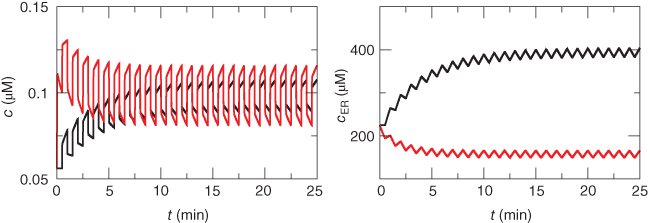
Figure 3.3 Depleting ER  (
( ) increases amplitude of cytosolic
  (
( ) response to pulses. Black: control, Red: SERCA (sarco-endoplasmic reticulum calcium ATPase) pump inhibited 50%. Equations and parameters as in Figure 3.2 but with
  pulsed between
  and
and  pA every 30 s.
Note that there are two time constants evident in Figure 3.3: with each pulse,  jumps up rapidly and then rises slowly. The rapid jumps reflect the fast intrinsic kinetics of
  , whereas the slow rise reflects the slow kinetics of
  , which pushes
  up slightly with each pulse as the ER fills. The slow kinetics of the ER are also manifest in the slow rise (black) and slow fall (red) of the envelope of
  as the ER fills or empties. The mean trend of
  , however, averaged over the rapid fluctuations, does approach approximately the same level irrespective of the fact whether the pump is inhibited or not. That is, Theorem 3.2.1 applies approximately to the averaged system.
3.3 ER-driven calcium oscillations
3.3.1 Closed cell
The model we have considered so far has a very limited repertoire because it is linear. There is a unique steady state, and the most the system can do is relax to that steady state exponentially or as a sum of exponentials. Put in other terms, the model has only negative feedback, embodied in the SERCA and PMCA pumps, which suppresses any fluctuation of  away from rest. There is a strongimperative to keep
  stable, but some cells have evolved the ability to generate and profit from controlled large excursions away from rest. In order to obtain more dynamic responses, we need to make the model nonlinear, specifically to add positive feedback. We do this by postulating that
  increases the flux out of the ER, often referred to as “calcium-induced calcium release” (CICR). Moreover, the negative feedback, which is needed to limit and terminate the excursions, has to develop slowly enough that it does not cancel out the rise in
  too soon. We have already encountered examples of oscillations mediated by fast positive feedback combined with slow negative feedback in Chapter 1, McCobb and Zeeman, and Chapter 2, Bertram et al., where they were the bases of action potentials. Indeed, the model we introduce here has much in common with those electrical oscillators, though it works via
  rather than the membrane potential.
IP3 regulation of ER 
A simple example of cytosolic  oscillations is the model of Li and Rinzel (1994), which is a simplification of the model of DeYoung and Keizer (1992). This will serve as an exemplar of a wide class of models based on the IP3 receptor (IP3R), an internal receptor located on the ER membrane, which opens in response to the second messenger IP3. IP3 in turn is produced by the activation of a G-protein-coupled receptor (GPCR) on the plasma membrane that responds to an external signal, such as acetylcholine or GnRH; the GPCR is coupled to phospholipase C via G
 , which forms IP3 from phosphatidylinositol 4,5-bisphosphate (PIP2). The IP3R is moreover a ligand-gated
  channel; IP3 opens the channel and allows
  to flow down its concentration gradient from the ER to the cytosol. Thus, one way to introduce positive feedback is to assume that IP3 production is stimulated by rises in
  . This was the basis of the earliest models for
  oscillations (Meyer and Stryer, 1988; Swillens and Mercan, 1990). DeYoung and Keizer, in contrast, motivated by reports that
  could oscillate even when IP3 is held fixed, proposed that
  enhanced the activity of the IP3R directly. Both effects of
  are known to exist, and there has been a long, yet unresolved debate about which is more important, or whether they each occur in different types of
  oscillations. We will not enter that debate here, but simply use the hypothesis of DeYoung and Keizer as a learning tool.
Modeling the role of IP3
Bezprozvanny et al. (1991) showed that the steady state open probability of the IP3R was a bell-shaped function of  , which suggested that
  in high concentrations inactivates the channel. DeYoung and Keizer proposed that this inactivation provides negative feedback beyond that of SERCA to terminate the
  spike, and that its time scale controls the period of the oscillation. They developed a model with eight states, for all the combinations of activating
  , activating IP3 and inactivating
  , bound or unbound.
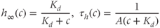
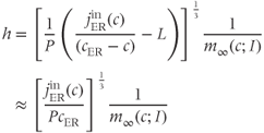
Li and Rinzel (1994) simplified this in the following formula:

where
 is the concentration of IP3, treated as a parameter; and
  is the fraction of available IP3 receptors, that is, the fraction not inactivated by binding
  .
.  satisfies the differential equation
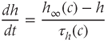
where
Equations (3.8) and (3.9) together say that the IP3R open probability is for fixed  an increasing function of [IP3] and
  , but decreases over time as receptors inactivate. This was deliberately formulated to highlight its similarity to the conductance of the voltage-dependent
  channel, described in Chapter 2, Equation (2.1), which increases with the membrane potential
  but inactivates over time.
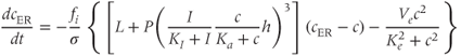
We can now assemble the pieces to specify the Li–Rinzel model, taking Equations (3.1) and (3.3) with Equation (3.8) in place of Equation (3.7) and
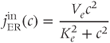
in place of Equation (3.6) (not strictly necessary but customary and more accurate). The equations for  and
and  then become
Finally, we add Equation (3.9) for receptor inactivation.
This system with three dependent variables ( ,
,  , and
, and  ) can be simplified by assuming that the cell is closed, that is, that the fluxes across the plasma membrane,
  and
and  are 0. This serves two purposes. First, it emphasizes that the oscillations only require flux in and out of the ER. Second, it reduces the number of equations to 2. The total
  content of the cell is

where  takes into account the differences in ER and cytosolic volume and buffering. This quantity is constant when the cell is closed: its time derivative is 0, as can be verified by multiplying Equation (3.3) by
  and adding to Equation (3.1). This reduction to two equations now allows us to use phase planes, shown in Figure 3.4, to understand the behaviors. (The concept and usage of phase planes are explained in Chapter 1, McCobb and Zeeman.)
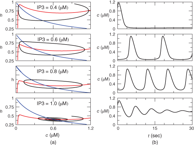
Figure 3.4 Phase planes (a) and timecourses (b) for the closed-cell Li–Rinzel model, Equations (3.9)–(3.11).  , fraction of IP3 receptors that are available to be opened (i.e. are not inactivated). Oscillations exist for an intermediate range of IP3 concentrations and, within that range, frequency increases with IP3. Parameters:
  as specified in the panels;
  ;
;  M/s;
M/s;  1/s;
1/s;  M;
M;  M;
M;  M/s;
M/s;  M;
M;  1/
1/ Ms;
Ms;  M;
M;  .
.
We solve the model equations for  and
and  (but can recover
  from Equation (3.12) should the need arise; see Figure 3.6). The left column shows the phase planes for three values of [IP3], and the right column shows the corresponding timecourses. The
  nullcline (blue) is obtained by setting the right-hand side of Equation (3.9) to 0 and solving for
  as a function of
  . It decreases monotonically, reflecting the increase of inactivation with
  (see Equation (3.9)).
The  nullcline (red) is obtained by setting the right-hand side of Equation (3.1) to 0. Conceptually, we want to solve for
  as a function of
  , but that equation can have up to three solutions for some values of
  , so it is easier to solve for
  as a function of
  . The
. The  nullcline is, thus, defined by
where we have neglected the small terms  and
and  in the second line (the latter is valid as long as
  is not too small). The resulting curve has a distorted N shape, increasing for small
  , then decreasing, and then increasing again. The left branch of the
  nullcline has a steep slope because
  as
as  . The N shape results from the competition between activation,
  , of the receptor, which increases
  , and SERCA,
  , which refills the ER. The general trend is for
  to increase due to SERCA, but in the range where the IP3R is strongly activated,
  turns down. This is typical for activator–inhibitor systems, where the positive feedback mechanism creates a kink in the activator variable nullcline and thereby creating instability and oscillations. In Hodgkin–Huxley-type systems, the activation of the
  current plays the same role. In that context, it creates a dip in the current–voltage relation, which translates to a negative resistance and gives away its role as the source of dynamism.
The intersection of the two nullclines is the steady state, and in each row there is only one. Increasing IP3 pulls down the  nullcline because
  is an increasing function of
  and moves the steady state along the
  nullcline. In the top row,
  M, the steady state is on the rising left branch of the
  nullcline, and is therefore stable. The trajectory (black) swings around from the upper right to end at the steady state, producing a single transient spike and then steady
  , as shown in the right panel. In this state, the system is not oscillatory but is said to be excitable, meaning that a suitable perturbation away from the rest state is amplified into a spike rather than returning immediately to rest.
For  M, the steady state is on the rising right branch of the
  nullcline and is again stable, but the approach to rest is a damped oscillation. In order to get sustained oscillations, the steady state must be destabilized, which is guaranteed if it lies on the falling middle branch of the
  nullcline. This is the case for
  M, shown in the middle panels. The trajectory now takes the form of a closed curve (a limit cycle, see Chapter 1, McCobb and Zeeman) that orbits around the steady state.
The phase plane also explains a characteristic feature of the oscillation, namely that the spikes are narrow and the interspike intervals are long. This happens because the trajectory is closer to the unstable steady state during the interspike portion, and the flow is therefore slow. The period decreases markedly as IP3 is increased within the oscillatory range because the steady state moves to the right, away from the low  values traversed during the interspike period (compare
  M to
M to  M in Figure 3.4). Thus, it is not difficult for models like this to capture the frequency encoding observed experimentally as the IP3-generating stimulus is varied (Goldbeter et al., 1990).
If we stack a series of phase planes like those in Figure 3.4 and plot the values of  (the steady states as well as the minima and maxima of the periodic orbits when those are present), we get Figure 3.5. A similar picture would be obtained if
  were plotted against IP3, so we omit the third dimension. The line shows the steady states, solid and black for stable, dashed and red for unstable. The green dotted line shows the average
  during spiking, and the filled circles the amplitude of the oscillations, which exist for a range of values of IP3, or between lower and upper thresholds. Those thresholds are labeled “HB” for Hopf bifurcation, which indicates the particular way in which the steady state goes unstable (see Chapter 1, McCobb and Zeeman). The existence of upper and lower thresholds, dividing the system behaviors into off, oscillating and fully on, is a ubiquitous feature of activator–inhibitor systems.
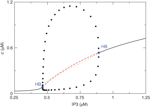
Figure 3.5 Bifurcation diagram for the closed-cell Li–Rinzel model. Oscillations in cytosolic  (
( ) exist for an intermediate range of IP3, demarcated by Hopf bifurcations (HB). Black: stable; lines: steady states; filled circles: min and max of oscillation; red: unstable steady states; green: average cytosolic
  during oscillations. Equations and parameters as in Figure 3.4
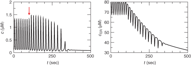
Figure 3.6 In the open-cell Li–Rinzel model (Equations (3.9), (3.13), (3.14)),  influx is needed to sustain oscillations. Parameters as in Figure 3.4 except:
  M;
M;  M/s;
M/s;  M;
M;  M;
M;  . We also add the plasma-membrane parameters:
  /s;
/s;  M; and
  , which is initially 2.5
  M/s and at
  s (red arrow) reduced to 0.
The peak  of the oscillation is in most cases higher than the steady
  level when
  is above the upper threshold, but the average is lower. The model thus suggests that if one could measure
  experimentally but not IP3, then the average would be a better indicator of the IP3 level (or “activity”) than the peak.
3.3.2 Open cell
Suppose now that the cell is open. Now during each  spike, some of the
  will be pumped out of the cell rather than back into the ER. Unless there is some
  influx to balance the efflux, the ER would eventually empty out and oscillations would cease. We restore the plasma-membrane fluxes, setting
  to a constant and introducing a saturating PMCA pump:
Related posts:
 Modeling Endocrine Cell Network Topology
Stay updated, free articles. Join our Telegram channel

Full access? Get Clinical Tree


