(a) The binomial distribution is the discrete probability distribution for the number of successes in a sequence of n independent success/failure experiments, each of which yields success with probability p. This plot shows that the probability of observing four successes among 35 trials assuming p = 0.2 is 0.082. (b, c) Unlike the binomial distribution, the normal and exponential probability distributions are used to describe continuous outcomes. The total area under these curves equals 1. Probabilities are defined in terms of areas under this curve. (b) The standard normal distribution assumes that the mean is 0 and the standard deviation is 1. The probability of observing an outcome greater than 2 is approximately 0.025, the area under the curve to the right of 2. The class of normal distributions can be generated by moving the location (mean) and stretching the distribution (standard deviation). (c) The standard exponential distribution assumes a rate of 1.
The binomial distribution is a discrete probability distribution for the number of successes in a sequence of n independent success/failure trials or experiments, where each individual trial yields success with probability p. This probability distribution can be used to describe outcome probabilities associated with the number of patients who respond to treatment in a clinical trial. Inference about p, the probability of success or response, is typically of primary interest.
The normal probability distribution is a commonly occurring continuous probability distribution that is informally referred to as a bell curve. The distribution is symmetric about the mean, and also characterized by the standard deviation, a measure of variability. Approximately 95% of observations for a normally distributed variable are within 2 standard deviations of the mean. Though many naturally occurring phenomena can be described by the normal distribution, this distribution is particularly useful because of the central limit theorem, which states that, under certain conditions, the distribution of a mean of many independent observations taken from the same distribution is approximately normal.
The exponential distribution is used to describe a process in which events (e.g., deaths) occur continuously and independently at a constant average rate. This distribution is particularly important in the context of survival analyses.
Estimation and hypothesis testing
Studies are typically conducted for one of two purposes: estimation or hypothesis testing. With estimation there is interest in obtaining an estimate or approximation for an unknown parameter, such as a mean, that characterizes a population based upon sample data. In conjunction with this estimate, a standard deviation or confidence interval is typically calculated that provides information about how well this sample statistic estimates the unknown population parameter. A confidence interval provides a range of values that is likely to contain the true population parameter of interest. Loosely, for a 95% confidence interval, we can say that we have 95% confidence that the true value of the parameter is within the calculated range. As the sample size increases, the precision of estimation typically increases, with a reduction in the width of the confidence interval as well as a reduction in the standard deviation associated with an estimate.
Alternatively, a study’s goal may be to assess a theory or hypothesis. When a statistical test is conducted, a null and an alternative hypothesis are stated with the goal of making a decision about which hypothesis is the most appropriate conclusion given available data. The alternative hypothesis reflects the theory that is to be proven. The features of a hypothesis test may be best explained through an example (Table 8.1). Consider a randomized study in which patients newly diagnosed with glioblastoma are randomized to receive standard-of-care treatment (temozolomide + radiation) with or without a novel treatment to ameliorate the cognitive effects of radiation treatment. The goal of the study is to show that the two arms differ with respect to the mean change in cognition. The null hypothesis, H0, is that the mean changes in cognition within the two arms are the same, and the alternative hypothesis, H1, is that the mean changes in the two arms are different. In conducting a statistical test of this hypothesis based upon available data, there are two types of potential errors: type I and type II. A type I error is committed when a conclusion is made that arms differ when they actually do not differ, and is considered to be a false-positive result. A type II error is committed when a conclusion is made that there are no differences when there truly are. Such an outcome is viewed as a false-negative result. The probability of a type I and II error are typically designated as α and β, respectively.
| Truth | |||
|---|---|---|---|
| True mean change in cognition same in both arms | True mean change in cognition different across arms | ||
| Conclusion | Mean change in cognition same in both arms | Correct decision | Type II error |
| Mean change in cognition different across arms | Type I error | Correct decision | |
The power of a statistical test is the probability of not committing a type II error (1 – β), or the probability that the alternative hypothesis is correctly accepted when the alternative hypothesis is true (i.e., 1 – β). In the context of the example study described above, it is the probability that one concludes that the treatments are different with respect to cognitive change when there is truly a difference. Power can be computed for any alternative.
As previously mentioned, the normal distribution is a probability distribution that appropriately describes many phenomena – but not all. Some of the more common basic statistical tests assume data are normally distributed, including the one-sample test, paired t-test, a two-sample t-test, and one-way analysis of variance (ANOVA).
One-sample t-tests assess hypotheses concerning the unknown population mean, where the mean is a measure of centrality for a normally distributed outcome or measure. As an example, a one-sample t-test would be appropriate if we want to determine whether an average brain cancer survivor has a normal IQ. In that case the null hypothesis is that the average IQ is 100 (i.e., H0: μ = 100, where μ is the unknown mean IQ) and the alternative hypothesis is that the average IQ is not 100 (i.e., H1: μ ≠ 100). The test statistic for this test is constructed as a ratio where the numerator is the difference between the parameter estimate and what it is hypothesized to be under the null hypothesis and the denominator is the standard deviation of the parameter estimate. In this case, the test statistic is:

where ¯x is the observed mean or parameter estimate, 100 is the hypothesized value of the true mean, and
 is the standard deviation of the mean, where s is the standard deviation of the data. If the test is conducted at the 0.05 level of significance, then the null hypothesis is rejected when |t| > t0.05/2, n–1 where t0.05/2,n–1 is obtained from the t-distribution with n–1 degrees of freedom. Statistical software will provide a p-value, the probability under the null hypothesis of observing a t statistic as extreme as that observed. An extremely rare event would be an indication that the null hypothesis is not true.
A paired t-test compares two sets of observations; however, these observations are not independent. Rather, there is a natural pairing between the two sets of observations. A prime example is a test to assess whether changes occurred over time in an outcome such as cognition (e.g., pre–post intervention). Of primary interest may be the change in cognition between a patient’s baseline assessment and a follow-up assessment within the same patient. What seems to be a two-sample problem can be converted to a one-sample assessment of a difference, or change in this example. A paired t-test is conducted by computing the paired difference and then conducting a one-sample t-test.
A two-sample t-test also compares two sets of observations; however, they are two independent sets of observations. The process for conducting a two-sample t-test is similar to that described for a one-sample t-test, except the parameter estimate is the observed mean difference and the standard deviation is a pooled estimate of the standard deviation within the two independent groups.
A one-way ANOVA compares the means of two or more groups of variables. A one-way ANOVA is equivalent to a two-sample t-test. The null hypothesis in a one-way ANOVA is that all groups have the same mean value, with the alternative being is that at least one mean is different from the others. An F-statistic is generated that is the ratio of the variance among the mean values and the variance across all data. A higher ratio implies that the samples were drawn from populations with different means.
Statistical methods have been developed that can assess the underlying assumptions for many of these statistical methods, including the normality assumption. If these underlying assumptions are not satisfied, alternative methods should be considered, including parametric models that are based upon a non-normal probability distribution, as well as non-parametric methods. Non-parametric methods make no assumptions about the underlying distribution of the variables being assessed. Some of the more common non-parametric tests are the Wilcoxon signed rank tests, the Wilcoxon rank sum test, and the Kruskal–Wallis test. These three tests are analogues to the parametric tests described above, and assess the location of the underlying data distribution. They are the non-parametric counterparts to the one-sample t-test, two-sample t-test, and one-way ANOVA, respectively. In these non-parametric tests, all collected data are ranked in some manner from smallest to largest and summed. Test statistics that are a function of these summed ranks are used to assess the test hypotheses concerning the location of the outcome distribution within the various groups. Statistical software will produce a test statistic and p-value. For small sample sizes, the p-value will probably be exactly computed as a permutation test. That approach involves computing the distribution of the test statistic under the null hypothesis by calculating all possible values of the test statistic under different arrangements of the observed ranks across groups. A p-value would represent the fraction of the frequency distribution of test statistics that are more extreme than the observed value.
Another notable parallel between parametric and non-parametric procedures is the correlation coefficient. A correlation coefficient measures the degree to which two characteristics vary together. A correlation ranges between –1 and 1, with a correlation of 0 indicating no association between the two variables, and correlations of –1 and 1 representing perfect negative or positive correlation. A Pearson correlation, which is a measure of linear relationship, requires normality for statistical testing. However, a Spearman correlation is a non-parametric assessment of association that is essentially a correlation of the ranked observations.
Concepts of sample size calculation
Early in the development of a clinical trial, discussions concerning sample size requirements commence. The resolution of those discussions is dependent upon various issues, including study design, study endpoint, study hypotheses, type I and type II error rates, and availability of financial and patient resources.
The approach to sample size calculation may differ slightly across study designs and endpoints; however, the concepts are similar. Consider the randomized study mentioned earlier in this chapter in which the mean cognitive changes in two groups of patients are compared. As already noted for this design, a two-sample t-test should be part of the study’s primary analysis. In determining the sample size requirements, questions that need to be asked include:
What is the magnitude of difference that would be important biologically or clinically to detect? What magnitude of difference would provide sufficient evidence to a clinical decision maker that the novel treatment has a role in the treatment of patients? The answer to these questions provides information about the difference for which the two-sample t-test should be powered to detect, and helps define the null and alternative hypothesis.
In the case of the two-sample t-test, what is a reasonable estimate for the standard deviation for change in cognition? A measure of variability is needed in the power calculation.
Many studies are designed with 80% power for a test conducted at the 0.05 level of significance. However, one could design the study with greater power or a larger type I error. It is important to consider whether a false-positive result or a false-negative result is of greater concern within the context of the specific study being designed. The challenge is that, as one controls either error rate with greater stringency, the sample size increases.
With this information one can determine the sample size for a two-sample t-test that would detect a clinically meaningful difference with the desired power and type I error rate. Unfortunately, the resulting sample size may not be feasible due to limited financial resources or issues regarding patient availability. As a result, the sample size determination process may become an iterative process. Type I or II error rates may be modified or the difference that the study is powered to detect may be modified to make the study feasible.
If modifications are required to make the study feasible prior to its initiation, there is a need to insure that the study will remain capable of providing meaningful results. Often there is a tendency to increase the difference between arms that is detectable with the chosen power level in order to reduce the sample size. The impact of this change is that the power to detect a clinically meaningful effect is reduced and the meaning of a negative study potentially compromised. If no difference between arms is ultimately observed during the study, one can conclude that there is no evidence of a difference. However, one cannot conclude that differences do not exist given the increased chance of committing a type II error when there are truly clinically meaningful differences. In other words, the study is underpowered to detect a clinically meaningful difference.
Multiple testing and interim analyses
We have considered errors associated with the conduct of one test. However, there are instances where multiple statistical tests may be of interest, either in the form of tests on several important outcome variables, or numerous interim analyses of the data. With each test that is conducted, there is a chance of committing an error, a type I error. If 100 tests are conducted at the 0.05 level of significance, one would expect that on average about five of these tests would be statistically significant when the null hypothesis is true. Controlling the family-wise error rate or overall type I error over all hypotheses conducted, or the false discovery rate (FDR), is often of interest. Numerous approaches for controlling the family-wise error rate have been proposed. Though rather conservative, the most common approach to managing the family-wise error rate is the Bonferroni correction, in which all tests are conducted at the α / m level of significance, assuming an overall type I error rate of α and m comparisons. FDR is a statistical method that controls the expected proportion of incorrectly rejected null hypotheses, or false discoveries.
In a similar vein, multiple looks at the same endpoint in the form of an interim analysis also inflate the type I error. Interim analyses should be prespecified in a protocol. Typically, the overall type I error will be partitioned among the interim and final analyses in order to maintain the overall α level.
Logistic regression
Often there is interest in understanding the factors that individually or collectively influence or are associated with outcome. If the outcome, Y, is normally distributed, multiple regression will often be considered to examine the impact of k predictors or explanatory variables [X =(x1, x2, x3, …, xk)] on that outcome:
However, if the outcome is a dichotomous outcome variable, logistic regression is commonly used. With such a model the impact of one or more explanatory variables on the probability, p, of a binary outcome variable (e.g., success or failure) can be examined. This model is derived from the logistic function that takes on values between 0 and 1 and has a sigmoidal shape (Figure 8.2).
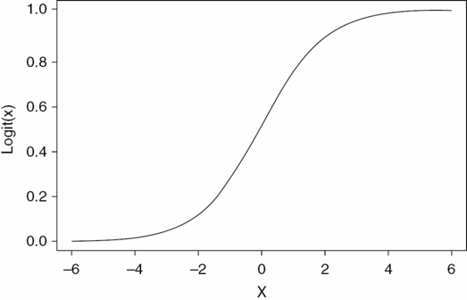
The logistic regression model is derived from the logistic function that takes on values between 0 and 1 and has a sigmoidal shape: f(x) = 1 / (1 + e–x).
A prime example might be a study where there is interest in exploring factors that might influence a patient’s response (e.g., responder or non-responder) to cancer therapeutic treatment. The linear logistic regression model describes the relationship between predictors and outcomes as follows:
where p is the probability of success and the βis are unknown covariable coefficients that are to be estimated from the data (Figure 8.2). More commonly, the model is reformulated to look somewhat like a multiple regression model using a logit function:
The slope coefficients or βs represent the change in the logit for a 1-unit change in the x. With this formulation being a function of an odds (i.e., p/(1 – p)), the βs also have an interpretation as the log odds ratio. The odds ratio is an important measure of association in epidemiology, as it estimates for a binary predictor how much more likely an outcome is present among those with x = 1, in contrast to those with x = 0.
Software packages are available that can be used to estimate the unknown coefficients within this model. These packages often use a maximum likelihood estimation algorithm. As with linear regression, the goal is to find the best-fitting and most parsimonious model that describes the relationship of interest. Many of the approaches to modeling used with linear regression are also applicable to logistic regression modeling.
Survival analysis
Some of the more important outcome measures in oncology are time to event outcomes, such as survival and progression-free survival. Survival or time to death is computed as the time between study entry and death. Progression-free survival is defined between study entry and death or initial disease progression. In most trials, complete follow-up is not available for all patients, as some patients will not have experienced the event that is of interest by the time of statistical analysis. For those patients, if survival is the event of interest, we know that the patient has lived at least as long as the time between entry and analysis time, and that death will occur at some point in the future. Survival time is censored at the time of last follow-up for such a patient. The product-limit estimator developed by Kaplan and Meier1 is a commonly used non-parametric estimate of the underlying survival curve, S(t), the probability that a patient’s survival is greater than t. The estimation procedure utilizes both censored and uncensored observations in the estimation of the survival curve.
To illustrate the computation of the Kaplan–Meier estimator, we will consider the following ordered survival times (in months) from 18 patients: 11, 13, 16, 16, 18, 21, 21, 22+, 23, 26+, 35, 36, 44, 47+, 48, 54+, 55+, 59+. Note that the “+” extension is the conventional approach to designating that the observation is censored. The calculation of Kaplan–Meier survival probabilities is demonstrated in Table 8.2. Within this table, the first column contains the time points at which the status of a patient changes (e.g., died or was censored). The second column provides information about the number of patients who were at risk of an event immediately prior to this time point. Columns 3 and 4 provide information about the type of event(s) that occurred at that time point. Within column 5, the proportion of patients surviving that time point among those who are at risk of dying at that particular time is computed. At month 11, 1 of the 18 patients at risk dies, with the surviving proportion being 0.994. At month 13, the probability of surviving is 0.889, which is the product of the probability of surviving 11 months (0.994) and the probability of surviving 13 months among those who survive 11 months (16/17). At month 22, a patient is censored. Given that the probability of surviving 22 months among those who survive 21 months is 1, the probability of surviving 22 months is the same as that at 21 months. The resulting Kaplan–Meier curve, as shown in Figure 8.3, is a step function.
| Time (months) | # at risk | # of deaths | # censored | Proportion surviving this time | Cumulative survival |
|---|---|---|---|---|---|
| 11 | 18 | 1 | 0 | 17 / 18 | 0.944 |
| 13 | 17 | 1 | 0 | 16 / 17 | 0.944 × (16 / 17) = 0.889 |
| 16 | 16 | 2 | 0 | 14 / 16 | 0.889 × (14 / 16) = 0.778 |
| 18 | 14 | 1 | 0 | 13 / 14 | 0.778 × (13 / 14) = 0.772 |
| 21 | 13 | 2 | 0 | 11 / 13 | 0.772 × (11 / 13) = 0.611 |
| 22 | 11 | 0 | 1 | 11 / 11 | 0.611 × (11 / 11) = 0.611 |
| 23 | 10 | 1 | 0 | 9 / 10 | 0.611 × (9 / 10) = 0.550 |
| 26 | 9 | 0 | 1 | 9 / 9 | 0.550 × (9 / 9) = 0.550 |
| 35 | 8 | 1 | 0 | 7 / 8 | 0.550 × (7 / 8) = 0.481 |
| 36 | 7 | 1 | 0 | 6 / 7 | 0.481 × (6 / 7) = 0.413 |
| 44 | 6 | 1 | 0 | 5 / 6 | 0.413 × (5 / 6) = 0.343 |
| 47 | 5 | 0 | 1 | 5 / 5 | 0.343 × (5 / 5) = 0.343 |
| 48 | 4 | 1 | 0 | 3 / 4 | 0.343 × (3 / 4) = 0.258 |
| 54 | 3 | 0 | 1 | 3 / 3 | 0.258 × (3 / 3) = 0.258 |
| 55 | 2 | 0 | 1 | 2 / 2 | 0.258 × (2 / 2) = 0.258 |
| 59 | 1 | 0 | 1 | 1 / 1 | 0.258 × (1 / 1) = 0.258 |
Stay updated, free articles. Join our Telegram channel

Full access? Get Clinical Tree


