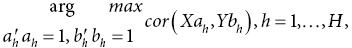
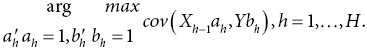
Statistical approaches to GSA

Despite the breadth of approaches to GSA, most methods can be broadly categorised as those based on over-representation; expression change scoring; or pathway topology. For an extended review of these approaches see Khatri et al. (2012).

Over-representation (OR) methods are the earliest examples of GSA. They are also arguably the simplest, and most broadly applicable across technological platforms. The general approach to OR proceeds as follows: first, a list of significantly regulated genes is determined from the microarray data using t-test, linear regression and so on, at a defined significance threshold. Next, the number of significant genes is counted both in the background list (often the entire microarray) and in each pre-defined gene set. Finally, each gene set is tested for significant enrichment with the genes of interest, typically using a test such as Fisher’s exact, hypergeometric, chi-square or binomial. The strength of the OR enrichment approach is in its simplicity. Using only a list of significant genes as input (without the need for fold change values or other quantitative measurements), this approach can be easily applied across a range of technological platforms, such as microarray, ChIP-on-chip, SNP array and so on. However, this simple use of gene lists also implies that OR approaches consider highly significant genes as identical to marginally significant genes, thus ignoring a potentially informative dimension of the data. Furthermore, the use of a significance threshold to define the initial gene list may exclude potentially informative genes that miss this threshold. Although there are relatively widely accepted standards for p-value thresholds in transcriptomic analysis, gene lists are often chosen also on the basis of fold change, for which there are fewer standards and which may or may not reflect true biological importance.

Expression change scoring (ECS) approaches inherently consider expression data in the calculation of gene set enrichment, and do not impose pre-selection of a significant gene list. The best-known example of an ECS approach was proposed by Subramanian et al. (who coined the initialism GSEA, for gene set enrichment analysis), with the original methodology paper receiving over 4000 citations to date (Subramanian et al. 2005). Similar to OR methods, ECS approaches to GSA begin with calculation of differential expression scores for each gene in the data set. These raw gene-level statistics may be used, or they may be transformed using absolute values, square root or rank statistics to remove the distinction between up- and downregulated genes (Subramanian et al. 2005; Saxena et al. 2006; Morine et al. 2010). These gene-level scores are then aggregated to gene set–level statistics, and the significance of each gene set is typically determined by a permutation test, either permuting the class labels or the gene labels.

One drawback of OR and ECS approaches, when applied to pathway gene sets, is that they do not consider the connectivity patterns between genes in each pathway. To illustrate the relevance of this information, consider the case of a very large pathway for which gene expression data have been measured across two conditions. It may be the case that the condition-specific expression changes in the pathway are localised to one small subregion, or alternatively they may be distributed evenly throughout the pathway. Pathway topology (PT)-based approaches were developed in an effort to capture this information in GSA. Current implementations use an ECS or OR approach to determine gene-level changes, then combine this statistic with gene–gene expression correlations (or a similar statistic) within the pathway (Rahnenführer et al. 2004; Tarca et al. 2009). The clear advantage of this approach is that it explicitly models pathway connectivity structure, which is a step closer to an understanding of dynamic system behaviour. However, it should be noted that the precise connectivity structure for many pathways is still only partially known, particularly when considering tissue- and cell type–specific activity.

Interpretation of GSA results

In the case of OR, ECS and PT approaches, the typical outcome of GSA is a list of gene sets that are significantly responsive to a perturbation or correlated with a particular phenotype. Depending on the database of gene sets used, this list of significant gene sets can become very long, containing hundreds or even thousands of gene sets. In this case, the problem of the lack of interpretability of high-throughput data is not resolved, only reduced. Furthermore, the list of significant gene sets often contains redundancies in terms of gene content (for instance, in the case of multiple related signalling pathways with a core set of shared genes). For this reason, a number of tools and approaches have been developed to aid in the interpretation and prioritisation of GSA results.

One such method, developed by Alexa et al. (2006) for the use of Gene Ontology (GO) terms as gene sets, involves explicit consideration of the GO structure in calculating GSA p-values for GO terms. The GO database is a controlled vocabulary for representing biological processes, functions and cellular compartments. It is structured as a directed acyclic graph, wherein the lower (child) nodes represent more specific biological categories, and each node inherits the categories of its parents. The entire collection thus appears as a hierarchy with a strong dependency structure between the nodes, in the sense that the majority of genes in a given child node will also be found in its parent node. Because of this dependency structure, any assumption of independence of gene sets is not valid. The methods proposed by Alexa et al. (2006) address this lack of independence in two ways. The first approach (called elim) examines the GO hierarchy from the bottom up, testing each GO term for significant enrichment with the given list of significant genes, then removing those genes from the parent terms if the tested child term is significantly enriched (essentially decorrelating the hierarchy). This approach favours the more specific child terms, which implicitly improves the interpretability of the results, as higher-level parent terms can become very broad in scope. In the second approach (called weight), significance scores of parent/child term pairs are compared, and the genes in the less significant term are downweighted. Although this second approach does not decorrelate the hierarchy, it enables local prioritisation among strongly dependent term pairs.

Another method for the interpretation and prioritisation of gene sets is called the leading-edge approach (Subramanian et al. 2007), which identifies gene sets containing the most highly scoring genes (i.e. the leading-edge subset). The implementation of this method allows for heatmap visualisation and calculation of correlation coefficients to assess the similarity between gene sets containing members of the leading-edge subset. Similar in concept to the approach of visualising the overlap between gene sets, the clueGO plugin (Bindea et al. 2009) for Cytoscape implements an OR approach to GSA and produces a network of enriched KEGG pathways of GO categories, wherein weighted links between gene sets represent the similarity between them, in terms of overlapping gene content.

The approaches already presented are relatively straightforward for the interpretation of data from simple study designs focusing on, for instance, a single nutrient/drug challenge or controls versus cases of a Mendelian disease. It is often the case in nutrition, however, that a researcher may be interested in the effects of a particular nutrient on a particular disease, and the high-throughput molecular changes that mediate the two. This complicates the interpretation of GSA results, because the gene sets that are most responsive to the nutritional intervention may not be those that are most strongly linked to the disease of interest (Morine et al. 2010). Furthermore, complex study designs involving multiple doses, time points and batches complicate the process of calculating a single statistic for each gene, as required by ECS approaches.

Cluster analysis

Cluster analysis is a widely used method for identifying groups of strongly correlated samples and/or variables in multivariate datasets. The most common methods for clustering methods, k-means and hierarchical clustering, are considered as unsupervised methods as they assume no prior knowledge of sample or variable classes. Hierarchical clustering does not assign observations to discrete clusters, but instead constructs a hierarchy of similarity, often visualised as a dendrogram. This can be achieved either through agglomerative clustering (identifying similar observations and building the hierarchy from the bottom up) or divisive clustering (starting with the complete data set, and successively dividing it into nested subfractions). In either case, a similarity metric is required to define the similarity between observations quantitatively. Common similarity metrics include Euclidean, Manhattan and Mahalanobis distance. Apart from the similarity metric, a linkage criterion is also required in order to define the distance between clusters of observations. This may be the distance between the closest two observations between two groups (single-linkage clustering); the farthest two observations (maximum linkage clustering); or the distance between the centroid of the two groups (average linkage clustering). Given the simplicity and speed of hierarchical clustering, it is generally worthwhile to apply multiple similarity and linkage metrics to examine the structure of the data fully and identify observations that may strongly influence the clustering result.

Unlike hierarchical clustering, k-means clustering produces a discrete assignment of observations to clusters. The algorithm for k-means clustering generally proceeds by selecting k initial cluster centres and assigning each observation to the closest centre. Once each observation has been assigned, new cluster centres are calculated and each observation is assigned again to its closest cluster; in this step, some observations will change cluster while others will remain the same. The step of cluster centre calculation and observation reassignment is repeated until no observation changes cluster. In the application of k-means clustering, it is typical to run the algorithm across a range of values of k, and assess the goodness of fit of each result to the data using a diagnostic such as the elbow method, an information criterion method such as Akaike’s Information Criterion, or the Gaussian approach proposed by Hamerly and Elkan (2003).

Principal component analysis

The best-known approach to dimensionality reduction is principal component analysis (PCA), first proposed by Karl Pearson (Pearson 1901), which identifies linear combinations of the variables in a multivariate data set that represent the variance structure in a smaller number of latent, orthogonal vectors. To illustrate with a simple example, consider a transcriptomic data set containing expression measurements for a large number of genes across a group of individuals. It may be the case that a subset of the genes displays strong correlation with each other, and thus could be represented by a composite (latent) variable that captures a large amount of the variance in these genes. The orthogonal transformation imposed by PCA is such that the first latent vector (first principal component) accounts for the largest amount of variability in the data set, with each successive component accounting for less variability and being uncorrelated to the rest (i.e. due to the orthogonality constraint). Plotting the samples in this low-dimensional space (on the first two principal components, for example) may reveal an informative grouping structure across the samples, such as grouping by dietary treatment, phenotype, gender and so on.

Canonical correlation analysis

As it is increasingly common to measure more than one omics data type on a given set of samples, methods for exploring correlation structure within and between two multivariate data sets are essential for efficient analysis and clear interpretation of these large data sets. Canonical correlation analysis (CCA), originally proposed by Hotelling (1936), uses a latent variable approach to identify low-dimensional correlations between two sets of continuous variables – that is, by identifying maximally correlated pairs of latent variables. CCA accepts as input two matrices, X of dimension n × p and Y of dimension n × q, both measured on the same n samples. The specific aim of CCA is to identify H pairs of loading vectors a_h and b_h of dimension p and q, respectively, that solve the objective function

where h is the chosen dimension of the solution, and the n-dimensional latent variables Xa_h and Yb_h denote the canonical variates. Analogous to PCA, the first dimension will represent the most strongly correlated canonical variates, with successive dimensions being progressively less correlated. Also similar to PCA, each pair of canonical variates is orthogonal to each other pair, which aids in the interpretability of CCA results as the variables represented on each dimension will be largely non-redundant (i.e. each dimension captures a unique subset of the data).

A fundamental limitation of CCA when applied to cases where p+q>>n (as is the case with high-throughput data) is that the solution of the objective function requires calculation of the inverse of the covariance matrices XX′ and YY′, which are singular in the case of p+q>>n and thus lead to non-unique solutions of the canonical variates. Because of this, a number of authors have proposed methods for penalising the covariance matrices to allow for reliable matrix inversion. A penalised version of CCA using a combination of ridge regression (also known as Tikhonov regularisation) and lasso (least absolute shrinkage and selection operator) shrinkage (Tibshirani 1996) was proposed by Waaijenborg and Zwinderman (2009). Briefly, ridge regression obtains non-singular covariance matrices XX′ and YY′ by imposing a weighting penalty on the diagonal of the covariance matrices, wherein highly correlated pairs of variables receive similar weights. Lasso shrinkage imposes an additional penalty that shrinks variables with low explanatory power to zero, and thus can be viewed as a variable-selection procedure.

Partial least squares regression

Partial least squares (PLS) regression aims to model the relationship between two data sets in a regression context, where one data set is considered as a predictor and the other as a response (Wold et al. 1984). An example of where this could be appropriate in nutritional genomics is the analysis of multivariate dietary intake data (predictor) and transcriptomic data (response), as in Morine et al. (2011). As with CCA, PLS takes as input two matrices, X of dimension n×p and Y of dimension n×q. Although there are a number of variants of PLS, the general approach seeks a decomposition of X and Y with p– and q-dimensional loading vectors to optimise the objective function

Note that the PLS algorithm seeks to maximise the covariance as opposed to correlation between the n-dimensional latent vectors, and performs the calculation based on the residual matrix X_h-1 as opposed to X, as with CCA. An attractive feature of PLS is that it does not require inversion of the covariance matrices and thus it can be applied in the case of p+q>>n. However, penalised versions of PLS have been proposed, using lasso or ridge in order to facilitate variable selection simultaneously with dimensionality reduction (Kim-Anh et al. 2008).

In addition to variation in the algorithm for PLS objective function optimisation (with NIPALS and SIMPLS being the most common; Alin 2009), a number of extensions to PLS have been proposed to facilitate its applicability to various data forms, such as canonical mode PLS (Lê Cao et al. 2009) and PLS discriminant analysis (Lê Cao et al. 2011).