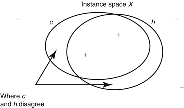
Learning capacity or “learnability” defines the ability of a machine-learning algorithm to learn the task at hand in terms of model complexity and the number of training samples required to optimize a performance criteria. Using formal statistical learning taxonomy [6], assuming a training set Ξ of n-dimensional vectors, , each labeled (by 1 or 0) according to a target function, f, which is unknown to the learner and called the target concept and is denoted by c, which belongs to the set of functions, C, the space of target functions as illustrated in Fig. 2.2. The probability of any given vector X being presented in Ξ is P(X). The goal of the training is to guess a function, h(X) based on the labeled samples in Ξ, called the hypothesis. We assume that the target function is an element of a set, H, the space of hypotheses. For instance, in our QA example, if we are interested in developing a treatment plan quality metric, we would have a list of input features X (e.g., energies, beam arrangements, monitor units, etc.) that is governed in our pool of treatment plans with a certain joint probability density function P. Based on clinical experience, a set of these plans are considered to be good while others are bad, which would constitute the target concept (c) of interest with an unknown functional form f that we aim to estimate. During the training process, we attempt to identify a hypothesis function h(X) that would approximate the mapping to c using varying possible machine-learning algorithms, and the higher the overlap between our hypothesized mapping function and the target quality metric concept, the more successful the learning process is as indicated in the Venn diagram of Fig. 2.2.

There are two main theories that attempt to characterize the learnability of machine-learning algorithms: the PAC and the VC theories as discussed below.

One method to characterize the learnability of a machine-learning algorithm is by number of training examples needed to learn a hypothesis h(X) as mentioned earlier. This could be measured by the probability of learning a hypothesis that is approximately correct (PAC). Formally, this could be defined as follows. Consider the concept class C defined over a set of instances X of length m and a learner L using hypothesis space H. C is PAC learnable by L using H.

If for all c ∈ C, distributions D over X, ε such that 0 < ε < 1/2 and δ such that 0 < δ < 1/2, there is a learner L with probability at least (1 – δ) that will output a hypothesis h ∈ H such that error D(h) ≤ ε, in time that is polynomial in 1/ε, 1/δ, n, and size (c) [4]. For a finite hypothesis space H, the number of training examples (m) required to reduce the probability of error below a desired level δ is given by assuming a zero training error:
This estimated number of training examples is sufficient to ensure that any consistent hypothesis will be probably (with probability (1 – δ)) approximately (within error ε) correct. In the case the training error is not necessarily zero, the number of required training examples becomes:
It is recognized that such estimate could be in practice an overestimate [4]. Another problem in PAC is that it includes the size of the hypothesis space H, which in practice could be infinite.

An alternative approach to measure learnability that overcomes the limitations of PAC is to use Vapnik–Chervonenkis (VC) dimension. The VC dimension measures the complexity of the hypothesis space H, not by the number of distinct hypotheses H as in PAC but rather by the number of distinct instances from X that can be completely discriminated using H. VC(H), of hypothesis space H defined over instance space X, is the size of the largest finite subset of X shattered by H. If arbitrarily large finite sets of X can be shattered by H, then VC(H) = ∞. This is noted that for any finite H, VC(H) ≤ log 2|H|. To see this, suppose that VC(H) = d. Then, H will require 2d distinct hypotheses to shatter d instances. Hence, 2 ^d  ≤ log 2|H|, and d = ≤ log 2|H|. This is illustrated in Fig. 2.2.