Classification of Malignant and Benign Tumors

(8.1)

where f(u, v) is a function determined using a machine learning approach, which we choose to be support vector machine (SVM) learning [26], and ζ is the modeling error. The similarity function f(u, v) in Eq. (8.1) is trained using data samples collected in an observer study.

8.2.2 Feature Extraction for Tumor Quantification

The purpose of feature extraction is to describe the content of a tumor under consideration by a set of quantitative descriptors, called features, denoted by vector x. Conceptually, these features should be relevant to the disease condition of the tumor. For example, they may be used to quantify the size of the tumor, the geometric shape of the tumor, the density of the tissue, etc., depending on the tumor type and specific application.

In the literature, there have been many types of features studied for classification of benign and malignant tumors. For example, in [27], effective thickness and effective volume were defined on the physical properties of MCs in mammogram images and were demonstrated to be useful for diagnosis. In [28], image intensity and texture features were extracted from post-contrast T1-weighted MR images and were shown to be helpful for brain tumor classification. In [29], wavelet features were compared with Haralick features [30] for MC classification.

While the reported features are many, they can be divided into two broad categories: (1) boundary-based features and (2) region-based features. Boundary-based features are used to describe the properties of the geometric boundary of a tumor. They include, for example, the perimeter, Fourier descriptors, and boundary moments [31]. In contrast, region-based features are derived from within a tumor region, which include the shape, texture, or the frequency domain information of the tumor. Some examples of region-based features are the tumor size, image moment features [31], wavelet-based features [29], and texture features [28].

To ensure good classification performance, the features extracted from a tumor are desired to have certain properties pertinent to the application. For example, a common requirement is that the features should be invariant to any translation or rotation in a tumor image. Other considerations in extracting or designing quantitative features include the effects of the image resolution and gray-level quantization used for the image. The image resolution can affect those features related to the size of a tumor, such as its area and perimeter. The quantization level in an image can affect those features related to the image intensity, such as image moments and features derived from the gray-level co-occurrence matrix (GLCM) [28]. Therefore, prior to feature extraction, the tumor images need to be preprocessed properly in order to avoid any discrepancy in resolution and quantization.

With a great number of features available, as described above, an important task in a CADx framework is how to determine a set of discriminative features in a tumor classification problem. These features are desired to have good differentiating power between benign and malignant tumors. One approach is to exploit the working knowledge of the clinicians and select those features that are closely associated with what the clinicians use in their diagnosis of the lesions [10]. For example, for MC lesions, the size and shape of the MCs and their spatial distribution are all known to be important, because the MCs tend to be more irregular and have a bigger cluster in a malignant lesion [13]. Alternatively, to determine the most salient features for use in the classification, one may employ a systematic feature selection procedure during the training stage of the classifier. The commonly used feature selection procedures in the literature include the filter algorithm [32], wrapper algorithm [33], and embedded algorithm [34].

8.2.3 Design of Decision Function Using Machine Learning

The problem of classifying benign or malignant tumors is a classical two-class classification problem, with benign tumors being one class and malignant ones being the other. For a given tumor characterized by its feature vector x, a decision function f(x) is designed to determine which class, malignant or benign, x belongs to. Naturally, a fundamental problem is how to design the decision function for a given tumor type. A common approach to this problem is to apply supervised learning, in which a pattern classifier is first trained on a set of known cases, denoted as $\left\{\left({x}_i,{y}_i\right),i=1,\dots, N\right\},$ where a training sample is described by its feature vector x _i, and y _iis its known class-label (1 for malignant tumor and −1 for benign tumor). Once trained, the classifier is applied subsequently to classify other cases (unseen during training).

Broadly speaking, depending on its mathematical form, the decision function f(x) is categorized into linear and nonlinear classifiers. A linear classifier is represented as

$f(x)={w}^Tx+b$

(8.2)

where w is the discriminant vector and b is the bias, which are parameters determined from the training samples. In contrast, a nonlinear classifier f(x) has a more complex mathematical form and is no longer a linear function in terms of the feature variables x. One such example is the feed-forward neural network, in which (nonlinear) sigmoid activation functions are used at the individual nodes within the network.

Because of their simpler form, linear classifiers are easier to train and less prone to over-fitting compared to their nonlinear counterpart. Moreover, it is often easier to examine and interpret the relationship between the classifier output and the individual feature variables in a linear classifier than that in a nonlinear one. Thus, linear classifiers can be favored for certain applications. On the other hand, because of their more complex form, nonlinear classifiers can be more versatile and achieve better performance than linear ones when the underlying decision surface between the two classes is inherently nonlinear in a given problem.

Regardless of their specific form, the classifier functions typically involve a number of parameters, which need to be determined before they can be applied to classifying an unknown case. There have been many different algorithms designed for determining these parameters from a set of training samples, which are collectively known as supervised machine learning algorithms.

Consider, for example, the case of linear classifiers in Eq. (8.2). The parameters w and b can be determined according to the following different optimum principles: (1) logistic regression [35], in which the log-likelihood function of the training data samples is maximized under a logistic probability model; (2) linear discriminant analysis (LDA) [36], in which the optimal decision boundary is determined under the assumption of multivariate Gaussian distributions for the data samples from the two classes; and (3) support vector machine (SVM) [37], in which the parameters are designed to achieve the maximum separation margin between the two classes (among the training samples).

Similarly, there also exist many methods for designing nonlinear classifiers. One popular type of nonlinear classifiers is the kernel-based methods [38]. In a kernel-based method, the so-called kernel trick is used to first map the input vector x into a higher-dimensional space via a nonlinear mapping; afterward, a linear classifier is applied in this mapped space, which in the end is a nonlinear classifier in the original feature space. One such example is the popular nonlinear SVM classifier. Other kernel-based methods include kernel Fisher discriminant (KFD), kernel principle component analysis (KPCA), and relevance vector machine (RVM) [39].

Another type of commonly used nonlinear CADx classifiers is the committee-based methods. These methods are based on the idea of systematically aggregating the output of a series of individual weak classifiers to form a (more powerful) decision function. Adaboost [40] and random forests [41] are well-known examples of such committee-based methods. For example, in Adaboost, the training set is modified successively to obtain a sequence of weak classifiers; the output of each weak classifier is adjusted by a weight factor according to its classification error on the training set to form an aggregated decision function [40].

8.2.4 CADx Classifier Training and Performance Evaluation

In concept, a CADx classifier should be trained and evaluated by using the following three sets of data samples: a training set, a validation set, and a testing set. The training set is used to obtain the model parameters of a classifier (such as w and b in the linear classifier in Eq. (8.2)). The validation set is usually independent from the training set and is used to determine the tuning parameters of a classifier if it has any. For example, in kernel SVM, one may need to decide the type of the kernel function to use. Finally, the testing set is used to evaluate the performance of the resulting classifier. It must be independent from both the training and validation sets in order to avoid any potential bias.

Ideally, when the number of available data samples is large enough, the training, validation, and testing sets in the above should be kept to be mutually exclusive. However, in practice, the data samples are often scarce, making it impossible to obtain independent training, validation, and testing sets, which is often true when clinical cases are used. To deal with this difficulty, a k-fold cross-validation procedure is often used instead. The procedure works as following: first, the available n data samples are divided randomly into k roughly equal-sized subsets; subsequently, each of the k subsets is held out in turn for testing while the rest $\left(k-1\right)$ subsets are used together for training. In the end, the performance is averaged over the k held-out testing subsets to obtain the overall performance. A special case of the k-fold cross-validation procedure is when

, which is also called a leave-one-out procedure (LOO). It is known that a smaller k yields a lower variance but also a larger bias in the estimated performance. In practice,

or 10 is often used as a good compromise in cross validation [42, 43].

When there are parameters needed to be tuned in a classifier model, a double loop cross-validation procedure [44] can be applied to avoid any potential bias. A double loop cross-validation procedure has a nested structure of two loops (the inner and outer loops). The outer loop is the same as the standard k-fold cross validation above, which is used to evaluate the performance of the classifier. The inner loop is to further perform a standard k′-fold cross validation using only the training set of samples in each iteration of the outer loop, which is used to select the tuning parameters.

For evaluating the performance of a CADx classifier, a receiver-operating characteristic (ROC) analysis is now routinely used. An ROC curve is a plot of the classification sensitivity (i.e., true-positive fraction) as the ordinate versus the specificity (i.e., false-positive fraction) as the abscissa. For a given classifier, an ROC curve is obtained by continuously varying the threshold associated with its decision function over its operating range. As a summary measure of overall diagnostic performance, the area under an ROC curve (denoted by AUC) is often used. A larger AUC value means better classification performance.

8.3 Application Examples in Mammography

8.3.1 Mammography

Mammography is an imaging procedure in which low-energy X-ray images of the breast are taken. Typically, they are in the order of 0.7 mSv. A mammogram can detect a cancerous or precancerous tumor in the breast even before the tumor is large enough to feel. Despite advances in imaging technology, mammography remains the most cost-effective strategy for early detection of breast cancer in clinical practice. The sensitivity of mammography could be up to approximately 90 % for patients without symptoms [45]. However, this sensitivity is highly dependent on the patient’s age, the size and conspicuity of the lesion, the hormone status of the tumor, the density of a woman’s breasts, the overall image quality, and the interpretative skills of the radiologist [46]. Therefore, the overall sensitivity of mammography could vary from 90 to 70 % only [47]. Moreover, it is very difficult to distinguish mammographically benign lesions from malignant ones. It has been estimated that one third of regularly screened women experience at least one false-positive (benign lesions being biopsied) screening mammogram over a period of 10 years [48]. A population-based study included about 27,394 screening mammograms that were interpreted by 1,067 radiologists showed that the radiologists had substantial variations in the false-positive rates ranging from 1.5 to 24.1 % [49]. Unnecessary biopsy is often cited as one of the “risks” of screening mammography. Surgical, needle-core, and fine-needle aspiration biopsies are expensive, invasive, and traumatic for the patient.

8.3.2 Computer-Aided Diagnosis (CADx) of Microcalcification Lesions in Mammograms

Clustered microcalcifications (MCs) can be an important early sign of breast cancer in women. They are found in 30–50 % of mammographically diagnosed cases. MCs are calcium deposits of very small dimension and appear as a group of granular bright spots in a mammogram (e.g., Fig. 8.1). Because of their subtlety in appearance in mammogram images, accurate diagnosis of MC lesions as benign or malignant is a very challenging problem for radiologists. Studies show that a false-positive diagnostic imaging study leads to unnecessary biopsy of benign lesions, yielding a positive predictive value of only 20–40 % [50].

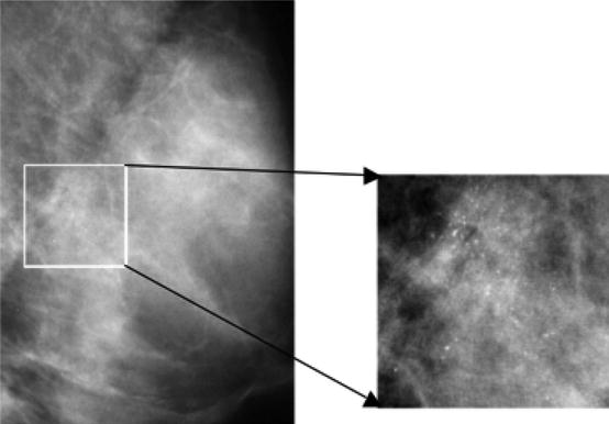
Fig. 8.1

A mammogram image (left) and its magnified view (right), where MCs are visible as granular bright spots

Because of their importance in cancer diagnosis, there has been intensive research in the development of CADx techniques for clustered MCs, of which the purpose is to provide a second opinion to radiologists in their diagnosis to improve the performance and efficiency [18]. In the literature, various machine learning methods such as LDA, logistic regression, ANN, and SVM have been used in the development of CADx classifiers for clustered MCs. For example, in [51], an LDA classifier was used for classification of benign and malignant MCs based on their visibility and shape features. This approach was subsequently extended to morphology and texture features in [52]. In [53], it was demonstrated an ANN-based approach could improve the diagnosis performance of radiologists for MCs. In [13], FKD, ANN, SVM, RVM, and committee machines were explored in a comparison study, wherein the SVM was shown to yield improved performance over the others. Collectively, the reported research results demonstrate that CADx has the potential to improve the radiologists’ performance in breast cancer diagnosis [54].

In the development of CADx techniques in the literature, various types of features have been investigated for characterizing MC lesions [9, 16, 55–58]. These features are defined to characterize the gray-level properties (e.g., the brightness, contrast, and gradient of individual MCs and the texture in the lesion region) or geometric properties of the MC lesions (e.g., the size and shape of the individual MCs, the number of MCs, the area, shape, and spatial distribution of a cluster). They are extracted either from the individual MCs or the entire lesion region. The features from individual MCs are often summarized using statistics to characterize an MC cluster.

CADx Example: Machine Learning Methods for MC Classification

In this section, we demonstrate the use of two CADx classifiers for clustered MCs, one is a linear classifier based on logistic regression, and the other is a nonlinear SVM classifier with a RBF kernel [13]. In logistic regression, the parameters w and b in Eq. (8.2) are determined through maximization of the following log-likelihood function:

$L\left(w,b\right)={\displaystyle \sum}_{i=1}^N \log p\left({y}_i,{x}_i;w,b\right)$

(8.3)

where the probability term is given by

$p\left({y}_i=1,\ {x}_i;w,\ b\right)={\left[1+ exp\left(-{w}^T{x}_i-b\right)\right]}^{-1}.$

(8.4)

For the nonlinear SVM classifier, it can be represented as

$f(x)={w}^T\varPhi (x)+b$

(8.5)

where w is the discriminant vector, b is the bias, and Φ(x) is a nonlinear mapping function which is implicitly defined by a kernel function (RBF in our case).

Based on the maximum marginal criterion, the parameters w and b in (8.5) are determined as following:

$\begin{array}{l} \min J\left(w,\xi \right)=\frac{1}{2}{\left|\left|w\right|\right|}^2+C{\displaystyle \sum}_{i=1}^N{\xi}_i\hfill \\ {}\mathrm{s}.\mathrm{t}.\kern0.24em {y}_if\left({x}_i\right)\ge 1-{\xi}_i,{\xi}_i\ge 0,i=1,2,\cdots, N\hfill \end{array}$

(8.6)

For testing these classifiers, we used a dataset of 104 cases (46 malignant, 58 benign), all containing clustered MCs. This dataset was collected at the University of Chicago. It contains some cases that are difficult to classify; the average classification performance by a group of five attending radiologists on this dataset yielded a value of only 0.62 in the area under the ROC curve [10]. The MCs in these mammograms were marked by a group of expert readers.

For this dataset, a set of eight features were extracted to characterize MC clusters [10]: (1) the number of MCs in the cluster, (2) the mean effective volume (area times effective thickness) of individual MCs, (3) the area of the cluster, (4) the circularity of the cluster, (5) the relative standard deviation of the effective thickness, (6) the relative standard deviation of the effective volume, (7) the mean area of MCs, and (8) the second highest shape-irregularity measure. These features were selected such that they have meanings that are closely associated with features used by radiologists in clinical diagnosis of MC lesions.

To evaluate the classifiers, a leave-one-out (LOO) procedure was applied to the 104 cases, and the ROCKIT software was used to calculate the performance AUC. The logistic regression classifier achieved AUC = 0.7174. In contrast, the SVM achieved AUC = 0.7373. These results indicate that the classification performance of the classifiers is far from being perfect, which illustrates the difficulty in diagnosis of MC lesions in mammograms.

8.3.3 Adaptive CADx Boosted with Content-Based Image Retrieval (CBIR)

In recent years, CBIR has been studied as a diagnostic aid in tumor classification [59, 60], of which the goal is to provide radiologists with examples of lesions with known pathology that are similar to the lesion being evaluated. A CBIR system can be viewed as a CADx tool to provide evidence for case-based reasoning. With CBIR, the system first retrieves a set of cases similar to a query, which can be used to assist a decision for the query [61]. For example, in [62, 63], the ratio of malignant cases among all retrieved cases was used as a prediction for the query. In [64], the similarity levels between the query and retrieval cases were used as weighting factors for prediction.

We have been investigating an approach of using retrieved images to boost the classification of a CADx classifier [65–67]. In conventional CADx, a pattern classifier was first trained on a set of training cases and then applied to subsequent testing cases. Deviating from approach, for a given case to be classified (i.e., query), we first obtain a set of known cases with similar features to that of the query case from a reference database and use these retrieved cases to adapt the CADx classifier so as to improve its classification accuracy on the query case. Below, we illustrate this approach using a linear classifier with logistic regression [65].

Assume that a baseline classifier f(x) in the form of Eq. (8.2) has been trained with logistic regression as in Eq. (8.2) on a set of training samples: $\left\{\left({x}_i,{y}_i\right),i=1,\dots, N\right\}.$ Now, consider a query lesion x to be classified. Let $\left\{\left({x}_i^{(r)},{y}_i^{(r)}\right),i=1,\dots, {N}_r\right\}$ be a set of N _rretrieved cases which are similar to x. In our case-adaptive approach, we use the retrieved samples $\left\{\left({x}_i^{(r)},{y}_i^{(r)}\right),i=1,\dots, {N}_r\right\}$ to adapt the classifier f(x). Specifically, the objective function in (8.3) is modified as

$L\left(w,b\right)={\displaystyle \sum}_{i=1}^N \log p\left({y}_i,{x}_i;w,b\right)+{\displaystyle \sum}_{i=1}^{N_r}{\beta}_i \log p\left({y}_i^{(r)},{x}_i^{(r)};w,b\right)$

(8.7)

In (8.7), the weighting factors β _iare adjusted according to the similarity of x _i^(r) to the query x. The idea is to put more emphasis on those retrieved samples that are more similar to the query, with the goal of refining the decision boundary of the classifier in the neighborhood of the query. Indeed, the first term in (8.7) simply corresponds to the log-likelihood function in (8.3), while the second term can be viewed as a weighted likelihood of those retrieved similar samples. Intuitively, the retrieved samples are used to steer the pretrained classifier from (8.3) to achieve more emphasis in the neighborhood of the query x. Note that the objective function in (8.7) has the same mathematical form as that in the original optimization problem in (8.3), which can be solved efficiently by the method of iteratively reweighted least square (IRLS) [35].

In our study, we implemented the following strategy for adjusting β _iaccording to the similarity level of a retrieved sample x _i^(r) to the query x:

${\beta}_i=1+k\frac{\alpha_i}{\underset{j=1,\dots, {N}_r}{ \max}\left\{{\alpha}_j\right\}},\kern0.46em i=1,\dots, {N}_r$

(8.8)

where α _idenotes the similarity measure between x _i^(r) and x, and $$ k>0 $$
” src=”/wp-content/uploads/2016/10/A320877_1_En_8_Chapter_IEq8.gif”></SPAN> is a parameter used to control the degree of emphasis on the retrieved samples relative to other training samples. The choice of the form in Eq. (<SPAN class=InternalRef><A href=

$$ k>0 $$
” src=”/wp-content/uploads/2016/10/A320877_1_En_8_Chapter_IEq8.gif”></SPAN> is a parameter used to control the degree of emphasis on the retrieved samples relative to other training samples. The choice of the form in Eq. (<SPAN class=InternalRef><A href=

8.8) is such that the weighting factor increases linearly with the similarity level of a retrieved case to x, with the most similar case among the retrieved receiving maximum weight $$ 1+k $$