Chance

It is a common practice to judge a result significant, if it is of such a magnitude that it would have been produced by chance not more frequently than once in twenty trials. This is an arbitrary, but convenient, level of significance for the practical investigator, but it does not mean that he allows himself to be deceived once in every twenty experiments.

—Ronald Fisher 1929 (1)

Learning from clinical experience, whether during formal research or in the course of patient care, is impeded by two processes: bias and chance. As discussed in Chapter 1, bias is systematic error, the result of any process that causes observations to differ systematically from the true values. Much of this book has been about where bias might lurk, how to avoid it when possible, and how to control for it and estimate its effects when bias is unavoidable.

On the other hand, random error, resulting from the play of chance, is inherent in all observations. It can be minimized but never avoided altogether. This source of error is called “random” because, on average, it is as likely to result in observed values being on one side of the true value as on the other.

Many of us tend to underestimate the importance of bias relative to chance when interpreting data, perhaps because statistics are quantitative and appear so definitive. We might say, in essence, “If the statistical conclusions are strong, a little bit of bias can’t do much harm.” However, when data are biased, no amount of statistical elegance can save the day. As one scholar put it, perhaps taking an extreme position, “A well designed, carefully executed study usually gives results that are obvious without a formal analysis and if there are substantial flaws in design or execution a formal analysis will not help” (2).

In this chapter, we discuss chance mainly in the context of controlled clinical trials because it is the simplest way of presenting the concepts. However, statistics are an element of all clinical research, whenever one makes inferences about populations based on information obtained from samples. There is always a possibility that the particular sample of patients in a study, even though selected in an unbiased way, might not be similar to the population of patients as a whole. Statistics help estimate how well observations on samples approximate the true situation.

TWO APPROACHES TO CHANCE

Two general approaches are used to assess the role of chance in clinical observations.

One approach, called hypothesis testing, asks whether an effect (difference) is present or is not by using statistical tests to examine the hypothesis
(called the “null hypothesis”) that there is no difference. This traditional way of assessing the role of chance, associated with the familiar “P value,” has been popular since statistical testing was introduced at the beginning of the 20th century. The hypothesis testing approach leads to dichotomous conclusions: Either an effect is present or there is insufficient evidence to conclude an effect is present.

The other approach, called estimation, uses statistical methods to estimate the range of values that is likely to include the true value—of a rate, measure of effect, or test performance. This approach has gained popularity recently and is now favored by most medical journals, at least for reporting main effects, for reasons described below.

HYPOTHESIS TESTING

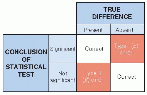
In the usual situation, the principal conclusions of a trial are expressed in dichotomous terms, such as a new treatment is either better or not better than usual care, corresponding to the results being either statistically significant (unlikely to be purely by chance) or not. There are four ways in which the statistical conclusions might relate to reality (Fig. 11.1).

Two of the four possibilities lead to correct conclusions: (i) The new treatment really is better, and that is the conclusion of the study; and (ii) the treatments really have similar effects, and the study concludes that a difference is unlikely.

False-Positive and False-Negative Statistical Results

There are also two ways of being wrong. The new treatment and usual care may actually have similar effects, but it is concluded that the new treatment is more effective. Error of this kind, resulting in a “falsepositive” conclusion that the treatment is effective, is referred to as a type I error or α error, the probability of saying that there is a difference in treatment effects when there is not. On the other hand, the new treatment might be more effective, but the study concludes that it is not. This “false-negative” conclusion is called a type II error or β error—the probability of saying that there is no difference in treatment effects when there is. “No difference” is a simplified way of saying that the true difference is unlikely to be larger than a certain size, which is considered too small to be of practical consequence. It is not possible to establish that there is no difference at all between two treatments.

Figure 11.1 ▪ The relationship between the results of a statistical test and the true difference between two treatment groups. (Absent is a simplification. It really means that the true difference is not greater than a specified amount.)

Figure 11.1 is similar to 2 × 2 tables comparing the results of a diagnostic test to the true diagnosis (see Chapter 8). Here, the “test” is the conclusion of a clinical trial based on a statistical test of results from the trial’s sample of patients. The “gold standard” for validity is the true difference in the treatments being compared—if it could be established, for example, by making observations on all patients with the illness or a large number of samples of these patients. Type I error is analogous to a false-positive test result, and type II error is analogous to a false-negative test result. In the absence of bias, random variation is responsible for the uncertainty of a statistical conclusion.

Because random variation plays a part in all observations, it is an oversimplification to ask whether chance is responsible for the results. Rather, it is a question of how likely random variation is to account for the findings under the particular conditions of the study. The probability of error due to random variation is estimated by means of inferential statistics, a quantitative science that, given certain assumptions about the mathematical properties of the data, is the basis for calculations of the probability that the results could have occurred by chance alone.

Statistics is a specialized field with its own jargon (e.g., null hypothesis, variance, regression, power, and modeling) that is unfamiliar to many clinicians. However, leaving aside the genuine complexity of statistical methods, inferential statistics should be regarded by the non-expert as a useful means to an end. Statistical testing is a means by which the effects of random variation are estimated.

The next two sections discuss type I and type II errors and place hypothesis testing, as it is used to estimate the probabilities of these errors, in context.

Concluding That a Treatment Works

Most statistics encountered in the medical literature concern the likelihood of a type I error and are
expressed by the familiar P value. The P value is a quantitative estimate of the probability that differences in treatment effects in the particular study at hand could have happened by chance alone, assuming that there is in fact no difference between the groups. Another way of expressing this is that P is an answer to the question, “If there were no difference between treatment effects and the trial was repeated many times, what proportion of the trials would conclude that the difference between the two treatments was at least as large as that found in the study?”

In this presentation, P values are called P_a, to distinguish them from estimates of the other kind of error resulting from random variation, type II errors, which are referred to as P_β. When a simple P is found in the scientific literature, it ordinarily refers to P_α.

The kind of error estimated by P_α applies whenever one concludes that one treatment is more effective than another. If it is concluded that the P_α exceeds some limit (see below) so there is no statistical difference between treatments, then the particular value of P_α is not as relevant; in that situation, P_β (probability of type II error) applies.

Dichotomous and Exact P Values

It has become customary to attach special significance to P values below 0.05 because it is generally agreed that a chance of <1 in 20 is a small enough risk of being wrong. A chance of 1 in 20 is so small, in fact, that it is reasonable to conclude that such an occurrence is unlikely to have arisen by chance alone. It could have arisen by chance, and 1 in 20 times it will, but it is unlikely.

Differences associated with P_α < 0.05 are called statistically significant. However, setting a cutoff point at 0.05 is entirely arbitrary. Reasonable people might accept higher values or insist on lower ones, depending on the consequences of a false-positive conclusion in a given situation. For example, one might be willing to accept a higher chance of a false-positive statistical test if the disease is severe, there is currently no effective treatment, and the new treatment is safe. On the other hand, one might be reluctant to accept a false-positive test if usual care is effective and the new treatment is dangerous or much more expensive. This reasoning is similar to that applied to the importance of false-positive and false-negative diagnostic tests (Chapter 8).

To accommodate various opinions about what is and is not unlikely enough, some researchers report the exact probabilities of P (e.g., 0.03, 0.07, 0.11), rather than lumping them into just two categories (≤0.05 or >0.05). Users are then free to apply their own preferences for what is statistically significant. However, P values >1 in 5 are usually reported as simply P > 0.20, because nearly everyone can agree that a probability of a type I error >1 in 5 is unacceptably high. Similarly, below very low P values (e.g., P < 0.001) chance is a very unlikely explanation for an observed difference, and little further information is conveyed by describing this chance more precisely.

Another approach is to accept the primacy of P ≤ 0.05 and describe results that come close to that standard with terms such as “almost statistically significant,” “did not achieve statistical significance,” “marginally significant,” or “a trend.” These valueladen terms suggest that the finding should have been statistically significant but for some annoying reason was not. It is better to simply state the result and exact P value (or point estimate and confidence interval, see below) and let the reader decide for him or herself how much chance could have accounted for the result.

Statistical Significance and Clinical Importance

A statistically significant difference, no matter how small the P, does not mean that the difference is clinically important. A P value of <0.0001, if it emerges from a well-designed study, conveys a high degree of confidence that a difference really exists but says nothing about the magnitude of that difference or its clinical importance. In fact, trivial differences may be highly statistically significant if a large enough number of patients are studied.

Example

The drug donepezil, a cholinesterase inhibitor, was developed for the treatment of Alzheimer disease. In a randomized controlled trial to establish whether the drug produced worthwhile improvements, 565 patients with Alzheimer disease were randomly allocated to donepezil or placebo (3). The statistical significance of some trial end points was impressive: Both the mini-mental state examination and the Bristol Activities of Daily Living Scale were statistically different at P < 0.0001. However, the actual differences were small, 0.8 on a 30-point scale for the mini-mental state examination and 1 on a 60-point scale for the Bristol Activities of Daily Living Scale. Moreover, other outcomes, which more closely represented the burden of illness and care of these patients, were similar in the
donepezil and placebo groups. These included entering institutional care and progression of disability (both primary end points) as well as behavioral and psychological symptoms, caregiver psychopathology, formal care costs, unpaid caregiver time, and adverse events or death. The authors concluded that the benefits of donepezil were “below minimally relevant thresholds.”

On the other hand, very unimpressive P values can result from studies with strong treatment effects if there are few patients in the study.

Statistical Tests

Statistical tests are used to estimate the probability of a type I error. The test is applied to the data to obtain a numerical summary for those data called a test statistic. That number is then compared to a sampling distribution to come up with a probability of a type I error (Fig. 11.2). The distribution is under the null hypothesis, the proposition that there is no true difference in outcome between treatment groups. This device is for mathematical reasons, not because “no difference” is the working scientific hypothesis of the investigators conducting the study. One ends up rejecting the null hypothesis (concluding there is a difference) or failing to reject it (concluding that there is insufficient evidence in support of a difference). Note that not finding statistical significance is not the same as there being no difference. Statistical testing is not able to establish that there is no difference at all.

Some commonly used statistical tests are listed in Table 11.1. The validity of many tests depends on certain assumptions about the data; a typical assumption is that the data have a normal distribution. If the data do not satisfy these assumptions, the resulting P value may be misleading. Other statistical tests, called non-parametric tests, do not make assumptions about the underlying distribution of the data. A discussion of how these statistical tests are derived and calculated and of the assumptions on which they rest can be found in any biostatistics textbook.

Figure 11.2 ▪ Statistical testing.

Table 11.1 Some Statistical Tests Commonly Used in Clinical Research

Test	When Used
*To Test the Statistical Significance of a Difference*
Chi square (χ²)	Between two or more proportions (when there are a large number of observations)
Fisher’s exact	Between two proportions (when there are a small number of observations)
Mann-Whitney U	Between two medians
Student t	Between two means
F test	Between two or more means
*To Describe the Extent of Association*
Regression coefficient	Between an independent (predictor) variable and a dependent (outcome) variable
Pearson’s r	Between two variables
*To Model the Effects of Multiple Variables*
Logistic regression	With a dichotomous outcome
Cox proportional hazards	With a time-to-event outcome

The chi-square (χ²) test for nominal data (counts) is more easily understood than most and can be used to illustrate how statistical testing works. The extent to which the observed values depart from what would have been expected if there were no treatment effect is used to calculate a P value.

Example

Cardiac arrest outside the hospital has a poor outcome. Animal studies suggested that hypothermia might improve neurologic outcomes. To test this hypothesis in humans, 77 patients who remained unconscious after resuscitation from out-of-hospital cardiac arrest were
randomized to cooling (hypothermia) or usual care (4). The primary outcome was survival to hospital discharge with relatively good neurologic function.

Observed Rates

	Survival with Good Neurological Function
	Yes	No	Total
Hypothermia	21	22	43
Usual care	9	25	34
Total	30	47	77

Success rates were 49% in the patients treated with hypothermia and 26% in the patients on usual care. How likely would it be for a study of this size to observe a difference in rates as great as this or greater if there was in fact no difference in effectiveness? That depends on how far the observed results depart from what would have been expected if the treatments were of similar effectiveness and only random variation accounted for the different rates. If treatment had no effect on outcome, applying the success rate for the patients as a whole (30/77 = 39%) to the number of patients in each treatment group gives the expected number of successes in each group:

Expected Rates

	Success
	Yes	No	Total
Hypothermia	16.75	26.25	43
Usual care	13.25	20.75	34
Total	30	47	77

The χ² statistic is the square of the differences between observed and expected divided by expected, summarized over all four cells:

The magnitude of the χ² statistic is determined by how different all of the observed numbers are from what would have been expected if there were no treatment effect. Because they are squared, it does not matter whether the observed rates exceed or fall short of the expected. By dividing the squared difference in each cell by the expected number, the difference is adjusted for the number of patients in that cell.

The χ² statistic for these data is:

This χ² is then compared to a table (available in books and computer programs) relating χ² values to probabilities for that number of cells to obtain the probability of a χ² of 4.0. It is intuitively obvious that the larger the χ², the more likely chance is to account for the observed differences. The resulting P value for a chi-square test statistic of 4.0 and a 2 × 2 table was 0.046, which is the probability of a falsepositive conclusion that the treatments had different effects. That is, the study results meet the conventional criterion for statistical significance, P ≤ 0.05.

When using statistical tests, the usual approach is to test for the probability that an intervention is either more or less effective than another to a statistically important extent. In this situation, testing is called two-tailed, referring to both tails of a bell-shaped curve describing the random variation in differences between treatment groups of equal value, where the two tails of the curve include statistically unlikely outcomes favoring one or the other treatment. Sometimes there are compelling reasons to believe that one treatment could only be better or worse than the other, in which case one-tailed testing is used, where all of the type I error (5%) is in one of the tails, making it easier to reach statistical significance.

Concluding That a Treatment Does Not Work

Some trials are unable to conclude that one treatment is better than the other. The risk of a false-negative result is particularly large in studies with relatively few patients or outcome events. The question then arises: How likely is a false-negative result (type II or β error)? Could the “negative” findings in such
trials have misrepresented the truth because these particular studies had the bad luck to turn out in a relatively unlikely way?

Example

One of the examples in Chapter 9 was a randomized controlled trial of the effects on cardiovascular outcomes of adding niacin versus placebo in patients with lipid abnormalities who were already taking statin drugs (5). It was a “negative” trial: Primary outcomes occurred in 16.4% of patients taking niacin and 16.2% in patients taking placebo, and the authors concluded that “there was no incremental clinical benefit from the addition of niacin to statin therapy.” The statistical question associated with this assertion is: How likely was it that the study found no benefit when there really is one? After all, there were only a few hundred cardiovascular outcome events in the study so the play of chance might have obscured treatment effects. Figure 11.3 shows time-to-event curves for the primary outcome in the two treatment groups. Patients in the niacin and control groups had remarkably similar curves throughout follow-up, making a protective effect of niacin implausible.

Figure 11.3 ▪ Example of a “negative” trial. (Redrawn with permission from The AIM-HIGH Investigators. Niacin in patients with low HDL cholesterol levels receiving intensive statin therapy. N Engl J Med 2011;365:2255-2267.)

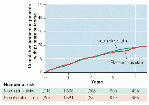
Visual presentation of negative results can be convincing. Alternatively, one can examine confidence intervals (see Point Estimates and Confidence Intervals, below) and learn a lot about whether the study was large enough to rule out clinically important differences if they existed.

Of course, reasons for false-negative results other than chance also need to be considered: biologic reasons such as too short follow-up or too small dose of niacin, as well as study limitations such as noncompliance and missed outcome events.

Type II errors have received less attention than type I errors for several reasons. They are more difficult to calculate. Also, most professionals simply prefer things that work and consider negative results unwelcome. Authors are less likely to submit negative studies to journals and when negative studies are reported at all, the authors may prefer to emphasize subgroups of patients in which treatment differences were found. Authors may also emphasize reasons other than chance to explain why true differences might have been missed. Whatever the reason for not considering the probability of a type II error, it is the main question that should be asked when the results of a study are interpreted as “no difference.”

HOW MANY STUDY PATIENTS ARE ENOUGH?

Suppose you are reading about a clinical trial that compares a promising new treatment to usual care
and finds no difference. You are aware that random variation can be the reason for whatever differences are or are not observed, and you wonder if the number of patients in this study is large enough to make chance an unlikely explanation for what was found. Alternatively, you may be planning to do such a study and have the same question. Either way, you need to understand how many patients would be needed to make a strong comparison of the effects of the two treatments?

Only gold members can continue reading. Log In or Register to continue