Chapter 1
Bridging Between Experiments and Equations: A Tutorial on Modeling Excitability
David P. McCobb1 and Mary Lou Zeeman2
1Department of Neurobiology and Behavior, Cornell University, Ithaca, NY, USA
2Department of Mathematics, Bowdoin College, Brunswick, ME, USA
The goal of this chapter is to empower collaboration across the disciplines. It is aimed at mathematical scientists who want to better understand neural excitability and experimentalists who want to better understand mathematical modeling and analysis. None of us need to be expert in both disciplines, but each side needs to learn the other’s language before our conversations can spark the exciting new collaborations that enrich both disciplines. Learning is an active process:
Tell me and I will forget; show me and I may remember; involve me and I will understand.
– Proverb
We have, therefore, written this chapter to be highly interactive. It is based on the classic model of excitability developed by Morris and Lecar (1981), and built around exercises that introduce the freely available dynamical systems software, XPP (Ermentrout, 2012), to explore and illustrate the modeling concepts. An online graphing calculator, such as Desmos (www.desmos.com), is also used occasionally. The modeling and dynamical systems techniques we develop are extremely versatile, with broad applicability throughout the sciences and social sciences. In the chapters of this volume, they are applied to systems at scales ranging from individual cells to entire neuroendocrine axes. We recommend that you work on the exercises as you read, with plenty of time, and tea and chocolate in hand. It is a great way to learn.
Outline. In Section 1.1, we introduce excitability, encompassing the diversity of action potential waveforms and patterns, recurrent firing, and bursting. We also describethe voltage clamp, the essential tool for dissection of excitability used by Hodgkin and Huxley (1952) in their foundational work. In Section 1.2, we introduce the classic, two-dimensional Morris–Lecar model, developed originally from barnacle muscle data to expose the minimal mathematical essence of excitability (Morris and Lecar, 1981). In Sections 1.3 and 1.4, we introduce the software package XPP (see Section 1.3 and Ermentrout (2012)) for download instructions), and use it to explore the model behavior, thereby introducing the language and graphics of dynamical systems and phase-plane analysis. This provides a platform for extending the model and including data from naturally occurring ion channels to dissect the excitability of diverse and more complex cells.
In Sections 1.5–1.10, we follow the seminal paper by Rinzel and Ermentrout (1989) to explore the surprising richness of behavior the Morris–Lecar model can exhibit in response to sustained current injection at various levels. We use three different parameter sets, differing only in the voltage dependence and kinetics of potassium channel gating. For each parameter set, we simulate a current clamp experiment in which sustained current is applied to a cell at rest. In all the three cases, sufficiently high levels of applied current induce tonic spiking, but the onset of spiking occurs through different mechanisms with different properties. With the first parameter set (“Hopf” in Table 1.1), tonic spiking is restricted to a narrow frequency range, as in Hodgkin’s Class II, typically resonator, neurons (Hodgkin, 1948). The second parameter set (“SNIC” in Table 1.1) exhibits tonic spiking with arbitrarily low frequency, depending on the applied current, as in Hodgkin’s Class I, typically integrator, neurons. The final parameter set (“Homoclinic” in Table 1.1) generates tonic spiking with a high baseline between the spikes. In Section 1.10, we exploit the high baseline to illustrate how adding a slow variable to the model can generate bursting behavior. Our tour of the Morris–Lecar model owes much to Rinzel and Ermentrout (1989) and many others, including Ellner and Guckenheimer (2006), Izhikevich (2007), Morris and Lecar (1981), and Sherman (2011).
Table 1.1 Variables and parameter values used
| Variable or | Definition | Units | Hopf | SNIC | Homo |
| parameter | values | values | values | ||
 | Time | ms | |||
 | Membrane voltage at time  | mV | |||
 | Proportion of K channels open at time  | ||||
 | Proportion of Ca channels open at steady state at voltage  | ||||
 | Proportion of K channels open at steady state at voltage  | ||||
 | Applied currenta |  A cm A cm | |||
 | Capacitancea |  F cm F cm | 20 | 20 | 20 |
 | Ca reversal potential | mV | 120 | 120 | 120 |
 | K reversal potential | mV |  |  |  |
 | Leak reversal potential | mV |  |  |  |
 | Maximal Ca conductancea | mS cm | 4 | 4 | 4 |
 | Maximal K conductancea | mS cm | 8 | 8 | 8 |
 | Leak conductancea | mS cm | 2 | 2 | 2 |
 | Voltage at half-activation of Ca channels | mV |  |  |  |
 | Spread (steepness  ) of ) of  | mV | 18 | 18 | 18 |
 | Voltage at half-activation of K channels | mV | 2 | 12 | 12 |
 | Spread (steepness  ) of ) of  | mV | 30 | 17 | 17 |
 | Rate constant for K-channel kinetics | ms | |||
 | Voltage dependence of K-channel kinetics | ms | |||
 | Rate constant for K-channel kinetics at half-activation voltage | 0.04 | 0.04 | 0.22 |
a Throughout the tutorial, we suppress the cm on current, capacitance, and conductance.
Mathematically, a qualitative change in system behavior, such as the onset of spiking arises through a bifurcation. Different mechanisms for the onset of spiking correspond to different bifurcations. We work through each of these bifurcations carefully, as they typify the mechanisms for generating oscillations in two-dimensional systems, they can underlie mechanisms in higher dimensional systems, and they recur throughout the text.
Our interdisciplinary conversations have led to a route through the mathematical material that may seem unusual. We have not begun with local linear stability theory, because our experience suggests that, while many experimentalists haveexcellent intuition about rates of change at their fingertips, the abstraction of eigenvalues presents a road block. (This is a natural consequence of the typical mathematics requirements for a biology degree.) We have chosen, instead, to harness the intuition about rates, and the visual intuition afforded by XPP, to develop an insight into the global nonlinear dynamics and bifurcations of the system. Only then we conclude with a discussion of the role eigenvalues play in determining local stability, and thereby signalling bifurcations. References are provided for the interested reader to learn more.
1.1 Introducing excitability
Action potentials: Decisive action and “information transportation”. Cellular excitability is defined as the ability to generate an action potential (or spike): an explosive excursion in a cell’s membrane potential (Figure 1.1). Its all-or-nothing aspect makes it decisive. Its propensity to propagate in space enables signal transmission in biological “wires” that are too small and electrically leaky to transmit a passive electrical signal over more than a millimeter or 2. Most cells have strong ionic gradients that are nearly, but imperfectly counterbalanced: a higher concentration of potassium ions (K ) inside than out, versus higher sodium (Na
 ), calcium (Ca
 ) and chloride (Cl
 ) concentrations outside than in. Higher “resting” permeabilities of the cell membrane to K and Cl result in a significant inside-negative resting potential (for largely historical reasons this is referred to as a hyperpolarized state). Action potentials are explosive excursions in the positive (depolarizing) direction from the resting potential, often reversing the polarity substantially (but still referred to as depolarizing).
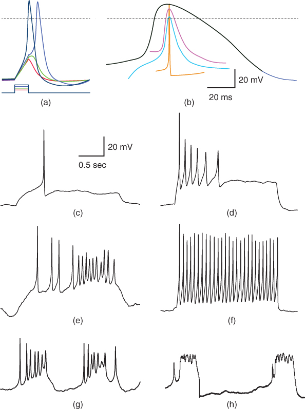
Figure 1.1 Variety of natural excitability. (a) Voltage responses of a mouse adrenal chromaffin cell to 10 ms current steps, recorded with whole-cell current clamp (McCobb Lab data). Action potential (AP) amplitudes were nearly invariant, and rise times varied modestly with stimulus amplitude. Voltage scale as in (b). (b) AP waveforms vary widely between cell types, ranging in duration from 180  s for a purkinje cell (orange; Bean (2007)) to
  ms for a cardiac muscle AP (black). Shown for comparison are spikes from a barnacle muscle cell (blue; Fatt and Katz (1953)) and a chromaffin cell (purple; McCobb Lab). (c–f) Patterns of spikes elicited with sustained current steps vary even between mouse chromaffin cells (McCobb Lab). Cell (c) would not fire more than one spike, (d) fired a train with declining frequency, amplitude, and repolarization rate, (e), an irregular volley, and (f), a very regular train at high frequency. (g, h) Pituitary corticotropes fire spontaneous bursts with features that vary between bursts and between cells, including spike amplitudes and patterns, as well as burst durations (McCobb Lab). Scale bars in (c) apply to (c–h).
The explosive mechanism uses positive feedback to produce a spatially regenerative event that propagates along a nerve axon, muscle fiber, or secretory cell’s membrane. Positive feedback arises from the fact that the opening of either sodium (Na) or calcium (Ca) ion channels (small selective and gated pores in the cell membrane) is (1) promoted by depolarization and (2) leads to further depolarization, as Na or Ca ions enter through the opened channels. The explosive depolarization can propagate at rates anywhere from 1 to 200 m/s (Xu and Terakawa, 1999) depending on cell specifics. This is very slow compared to the passive spread of a voltage signal in a metal wire (on the order of the speed of light!). It is limited by the time required for channels to respond to voltage, together with the effects of membrane capacitance and leak. Nevertheless, it is much faster than any other form of chemical or biochemical signal propagation, and fast enough to support animal life, including the transmission of information over some 2 million miles of axons in the human body.
The explosive, roughly all-or-nothing nature of the action potential also serves as a decisively thresholded regulator of Ca entry. It thereby regulates many precisely timed and scaled cellular events, including neurotransmitter and hormone secretion, muscle contraction, biochemical reactions, and evengene regulatory processes. Membrane voltage thus underlies rapid signal integration in the “biological computer,” including the regulation of neuroendocrine function.
For a cell to recover from the excursion from negative resting potential and prepare to fire another action potential, repolarization has to occur. This is achieved by combatting the positive feedback with slightly delayed negative feedback, or feedbacks. An essentially identical mechanism of depolarization-triggered opening of ion channels as described for Na or Ca, but now involving a channel type that selectively conducts K, quickly restores the hyperpolarized state. In response, the Na- or Ca-channel gates can now relax back to the closed state (as do the K-channel gates), a process referred to as deactivation. In most cases, the K-channel restorative mechanism is backed up by the closing of a separate inactivation gate within the body of the Na or Ca channel, which would prevent prolonged depolarization (and flooding of Na or Ca into the cell) even without the K channel. Together these events speed repolarization, deactivation and deinactivation (the reversal of inactivation). The separability of these gating events provides raw material for very sophisticated and sometimes subtle differences in firing and consequent signal integration.
Action potential shape and timing in information processing. Synaptic transmission is well known to play important roles in information processing. The details of intrinsic excitability of neuroendocrine cells are at least as important as in neurons, and even more so in cells like those in the anterior pituitary that are not directly driven by synaptic inputs. Thus, the variety, subtlety and susceptibility to modulatory changes of ion channels underlying excitability are critical to the nuances of neuroendocrine signalling. See Hille (2001), Chapter 7 in Izhikevich (2007) and Figure 1.1. Details of the rising phase control threshold and rise time, and influence frequency. The details of repolarization, recovery, and preparation for subsequent signalling events are even more nuanced and diverse, as indicated by the enormous diversity of K channels (at least an order of magnitude greater than that of Na and Ca channels). Action potential threshold, differing between cells, and depending on recent events and modulatory factors within a cell, determines whether a response is transmitted or squelched. It also contributes, as do ensuing features of the action potential, to the encoding of the stimulus strength as firing frequency. Spike amplitude shapes calcium channel activation and calcium entry, as well as K-channel activation. These in turn sculpt ensuing features, and, especially through calcium influx, sculpt the transduction from electrical response to output, including, for example, transmitter, modulator, hormone release, or muscle contraction. The latency of the rising phase is critical to encoding or integration, and can serve as a temporal filter. So, too, can the timing of repolarization and recovery. These can confer a resonance on the system that makes it selectively responsive to timing of input, and potentially, as responsive to hyperpolarizing as depolarizing input. Timing and the interplay between the channel mechanisms together pattern the timing of spikes. They can also confer intrinsic firing, exemplified by the beautifully complex rhythms of burst firing. In addition to influencing reactivity to inputs, intrinsic firing makes a neuron a potential source of action(or maintenance or inaction). Together the dimensions of complexity and variability that have evolved in electrical signalling contribute enormously to the intelligence of biological systems, including (but not exclusive to) the brain function.
Dissecting action potential mechanisms with voltage clamp. Hodgkin and Huxley (1952) used the voltage clamp to dissect the action potential in the squid giant axon. (The axon is a milimeter or more in diameter, roughly 100 times the diameter of the largest human fibers). This clever device measures the opening and closing of ion channels, as follows: the voltage difference between the inside and outside of an axon is measured, and compared to a desired or “command” voltage. Any discrepancy between measured and command potentials is then immediately eliminated by injecting current into the axon through a second internal electrode. The amount of current required to clamp the voltage depends on the membrane conductance (inverse of resistance), and thus changes as ion channels open or close (see Figure 1.2). While useful for studying any channels, the voltage clamp is especially important for voltage-gated channels. By varying the voltage itself in stepwise fashion, Hodgkin and Huxley were able to prove that the membrane had conductances that were directly gated by voltage. Then by removing Na and K ions independently, they resolved distinct inward and outward components, and noted their dramatically different kinetics. The inward (Na) current responded more rapidly, but terminated quickly, while the outward (K) current was slower but persisted. Recognizing that this voltage sensitivity might provide the feedback underlying the action potential, they carefully measured voltage- and time-dependent features, including activation and deactivation of inward and outward components, and inactivation and deinactivation of the inward component. They then constructed a mathematical model and solved it numerically for the response to a stimulus, with the similarity between the theoretical voltage response and a recorded action potential supporting the view that they had explained the basic mechanism.
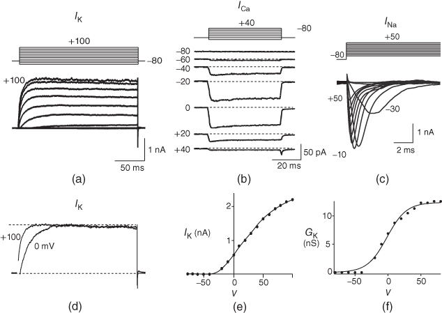
Figure 1.2 Voltage clamp data. (a, b, and c) Voltage-gated K, Ca, and Na currents, respectively, elicited with voltage steps in whole-cell voltage clamp mode applied to mouse chromaffin cells (McCobb Lab data). Outward currents are positive (upward), and inward currents are negative (downward). The K and Ca currents shown here exhibit little inactivation, though both types can inactivate in some chromaffin cells. The Na currents inactivate rapidly, and the current amplitude reverses sign when the test potential crosses the Na reversal potential. (d) K-current activation is faster at more depolarized potentials, as shown by normalizing the K currents at 0 and +100 mV from (a). (e) Current–voltage ( –
– ) plot for K currents from the cell in (a); peak current values are plotted against the corresponding test potential. (f) Conductance–voltage (
 –
– ) plot; current values from (e) are divided by the driving force (
 ) and plotted against test potential. The
  –
– curve gives a summary of the voltage dependence of gating without the confounding effect of driving force.
So why do we need to continue modeling action potentials and excitability? Hodgkin and Huxley (1952) predated the identification of ion channel proteins,
but their results implied sophisticated voltage-sensing and gating nuances, and gave birth to structure-function analysis with unprecedented temporal resolution. Action potentials in barnacle muscle, another early preparation, were shown to depend on Ca rather than on Na influx (Keynes et al., 1973). This laid the foundation for the Morris–Lecar model, in which one (excitatory) Ca current and one (repolarizing) K current interact to generate excitability (Morris and Lecar, 1981). Moreover, with glass electrodes enabling recordings in many more cell types, it became ever clearer that there was enormous variation on the general theme, begging further dissection. Every quantifiable feature of action potentials, from threshold to rise-time, duration, ensuing dip (afterhyperpolarization) and size, number, frequency, and pattern of additional action potentials elicited by various stimuli could be shown to vary from cell to cell. It is now clear that this variety sculpts signal input–output relationships for neurons and networks in almost limitless fashion. Meanwhile, a vast array of ion channel genes, accessory proteins, and modulatory mechanisms contributing to excitability has been identified (Coetzee et al., 1999; Dolphin, 2009; Hille, 2001; Jan and Jan, 2012; Jegla et al., 2009; Lipscombe et al., 2013; Zakon, 2012). A wealth of questions arise. How do structural elements and combinations encode functional nuances appropriate to physiological, behavioral, and ecological contexts in diverse animals? How did they arise through evolution? How they are coordinated in development? And how does event-sensitive plasticity contribute to adaptive modification of excitability-dependent computations? Relevant hypotheses clearly depend on theoretical dissection via mathematical modeling.
Why work with a model originating in barnacle muscle? Throughout the chapter, we will work with the Morris–Lecar model, which was originally developed for barnacle muscle and includes only two voltage-gated channel types (Ca and K), neither of which inactivates. Moreover, based on observations that showed the activation rate for the excitatory Ca current to be about 10-fold faster than that for the repolarizing K current and 20-fold faster than that for charging the capacitor (Keynes et al., 1973), Morris and Lecar (1981) simplified the model even further, reducing dimension by treating the Ca-channel activation as instantaneous.
You may ask why a neurobiologist or endocrinologist should spend time on such a simple system, so obviously peripheral to sophisticated neural computation. Or how simplification and omission justify the trouble of learning mathematical “hieroglyphics”. These questions raise the issue of what a mathematical model is good for. A powerful use of models is to help test hypotheses and design experiments about putative biological mechanisms underlying observed behaviors. To that end, minimal models, built from the ground up, allow for thorough dissection and attribution of mechanisms. For example, see Izhikevich (2007, Chapter 5) for a summary of six minimal models of excitability. After studying the Morris–Lecar model in this chapter, we hope that you will agree that what may at first look like an extremely limited system turns out to be capable of a surprisingly rich repertoire of waveforms and firing dynamics. Without studying such a minimal model, one might assume that more channel types or more complex gating mechanisms were needed to generate such a variety. After developing modeling confidence, it is easy to adjust parameters, or add inactivation, other channel types or gating mechanisms, as detailed in Chapter 2. The comparison between Morris–Lecar, Hodgkin–Huxley, and other model behaviors then helps to clarify the interactive mechanisms at play, and the roles of specific terms and parameters.
The reduced dimension of the Morris–Lecar model also provides an excellent starting point for model analysis. It allows us to explore and dissect the model behavior in a two-dimensional phase plane (detailed in Section 1.4), where, with the help of graphical software, we can harness our visual intuition to understand the concepts and language of dynamical systems. The dynamical systems approach is extremely versatile, generalizing to more complex models and higher dimensions, and highlighting similarities among mechanisms in a wide range of applications. Throughout this volume, we will see how dynamical analysis of minimal models, designed with the scale and complexity of the specific neuroendocrine question in mind, yields new biological insights.
1.2 Introducing the Morris–Lecar model
The Morris–Lecar model is discussed in many texts in mathematical biology and theoretical neuroscience. See, for example, Ellner and Guckenheimer (2006), Ermentrout and Terman (2010), Fall et al. (2005), Izhikevich (2007), and Koch (1999).
What is in the Morris–Lecar model? The model structure is represented by the circuit diagram in Figure 1.3a (Morris and Lecar, 1981). A system of Ca and K gradients with selective conductances provides “batteries” defining equilibrium or reversal potentials. There is also a “leak” of undefined (probably composite) conductance, with a measurable reversal potential. For our purposes, the chemical gradients do not change appreciably: ion pumps and exchangers work in the background to ensure this. Currents applied through the current electrode travel in parallel across the capacitor and any open ion channels or other leaks. Internal and external solutions offer no resistance to flow, so that the voltage across the capacitor and resistors/conductors in the membrane is equivalent. Moreover, the system is assumed to be spatially uniform; voltage over the entire membrane changes in unison. This fits well with data from compact neuroendocrine cells (Bertram et al., 2014; Liang et al., 2011; Lovell et al., 2004; Stojilkovic et al., 2010; Tian and Shipston, 2000).The approach is also useful for membrane patches in most neuronal contexts. Spatial nonuniformity and spatio-temporal propagation of signals are not addressed here.
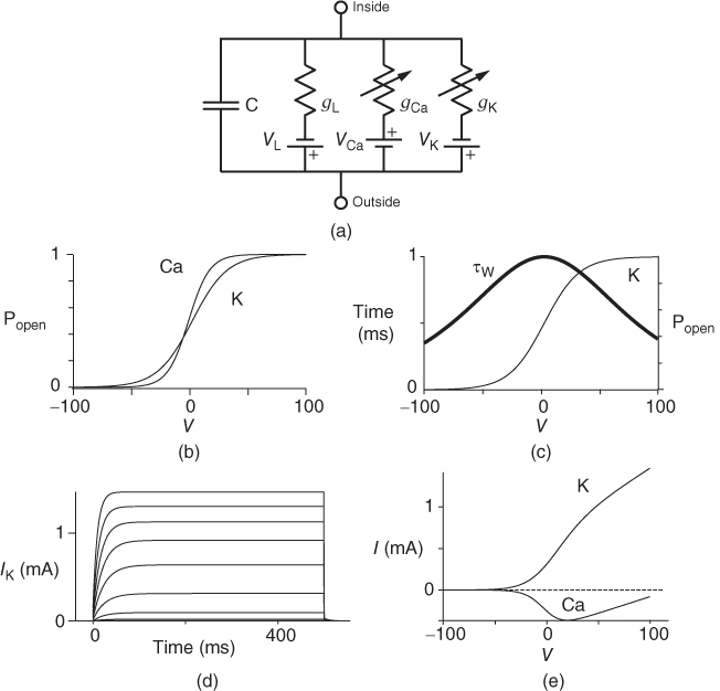
Figure 1.3 Morris–Lecar model. (a) Equivalent electrical circuit representation of the Morris–Lecar model cell. Membrane capacitance is in parallel with selective conductances and batteries (representing driving forces arising from ionic gradients). Arrows indicate variation (with voltage) for Ca and K conductance. (b) Normalized  –
– curves,
  and
and  , assumed for model K and Ca conductances, respectively. (c) The kinetics of voltage-dependent activation of K channels is also voltage dependent, with the normalized time constant,
  , assumed to peak (i.e., channel gating slowest) at the midpoint of the
  –
– curve, where channel conformational preference is weakest. (d) Simulated voltage clamped K currents at 20 mV increments up to
  =100 mV. Voltage clamp simulated in XPP by removing the equation for
  and, instead, setting
  as a fixed parameter. (e) Model
  –
– plots for K and Ca currents. Different reversal potentials for the two conductances (
 mV) make the current traces look very different, despite similar activation functions in (b). (b)–(e) Use Hopf parameter set.
What makes this an “excitable” membrane and an interesting dynamical system, is (1) feedback: the proportion of channels open (for both Ca and K channels) depends on voltage and (2) reactions of the channel gates to changes in voltage take time. Reaction rates also vary with voltage; but while this influences the voltage waveform, it is not essential for excitability.
Ion channel openings and closings are stochastic events, but their numbers are large enough that the currents associated with each type can be modeled as smooth functions. Thus, four variables interact dynamically:
- The voltage (transmembrane potential),
 , typically in millivolts, mV.
- The proportion of open channels,
 , for the voltage-gated Ca channel that drives the rising phase of the action potential. Since
  is a proportion, it ranges between 0 and 1, and has no units.
- The proportion of open channels,
 , for the voltage-gated K channel that terminates the action potential. Like
  ,
,  is a proportion, so ranges between 0 and 1.
- Time,
 , the independent variable, typically in milliseconds, ms.
Again, the dependent variables are functions of one another; they interact, and do so with time dependence. The rules by which they interact are translated into differential equations, as discussed below.
What is a differential equation? The only mathematical background we assume is that you have taken a calculus course sometime in the past (perhaps long ago) and remember (perhaps dimly) that the derivative represents instantaneous rate of change, or the slope of a graph. For example, Figure 1.1 shows several graphs of voltage,  versus time. Consider the detailed action potentials shown in Figure 1.1b. During the rising phase of each action potential, the slope of the graph is positive. So the derivative,
  , is positive. This is just another way of saying that
  is increasing or depolarizing. During the hyperpolarizing (decreasing) phase of each action potential, the graph is heading “downwards,” with a negative slope, so
  . At the peak of each action potential, a line tangent to the graph would be horizontal, with zero slope. So
  as the graph turns from increasing to decreasing. Similarly,
  as the graph turns from decreasing to increasing.
- (1.2.1) This is where the interactive part of the tutorial begins. This first exercise is designed to help cement the concepts of slope and derivative, and does not require any software. Choose one of the graphs in Figure 1.1 and track
 as you move along the graph. When is
  positive? When is it negative? How many times is it zero? When is
  greatest? When is it most negative? Try sketching the graph of
  below your graph of
  (it helps to have the time axes lined up).
A differential equation is just an equation with a derivative in it somewhere. Equation (1.1) is a differential equation relating the rate of change of voltage to the currents flowing through the cell membrane. The differential equation does not tell us about  directly, in the sense that it is not of the form
But if we can measure the value of  at one initial moment in time, Equation (1.1) tells us how
  will change, so that we can use it to predict all future values of
  . Adding up all the incremental changes in
  over time is called numerical simulation. It can be hard to do by hand, but is a job well suited to a computer. This is one of the reasons that mathematical modeling in biology has flourished with the computer revolution of recent decades, and why this tutorial is designed to be interactive, using the numerical simulation software XPP (Ermentrout, 2012).
A word of warning: the derivative is a fundamental concept in math ematics, so has earned many names;  (“
(“ by
by  ”),
”),  (“
(“ prime”), and
  (“
(“ dot”) are all equivalent in this context, and not to be confused with plain
  .
.
The differential equation for voltage change over time. According to Kirchoff’s current law, if a current  is applied across the membrane (through an electrode, say), it is balanced by the sum of the capitative and ionic currents:
If there is no applied current, then  . Here,
  and
and  denote the Ca and K currents respectively;
  denotes a leak current (a voltage independent current that may or may not be selective);
  denotes the capacitance, and
  represents the capacitive current. The fact that capacitive current is proportional to how quickly voltage changes
  is what makes this a differential equation. Rearranging to bring the derivative to the left-hand side,
Thus,

where the ionic currents are modeled by
Let us walk through these equations term by term, to understand the notation, and how the ionic currents are represented. To fix ideas, consider the K current. In Equation (1.3),  is modeled as the product of:
- The maximal K conductance,
 , that can be measured at any voltage (see Figure 1.2).
- The K-channel activation variable,
 , which changes over time (so is written
  , or
, or  for short). There is no K-channel inactivation in the model, so, relative to maximal conductance,
  represents the proportion of K channels that are open at time t, and the instantaneous probability that an individual K channel is in its open state. In other words,
  represents the normalized K conductance at time
  (taking values between 0 and 1), and
  represents the absolute K conductance. Expressions for the voltage dependence and kinetics of
  are formulated in Equations (1.6), (1.9), and (1.10).
- The driving force,
 , on K current through the K channels. This is the difference between
  of the moment and
  , the K reversal potential. The larger the difference, the larger the driving force; and as V changes over time, the driving force changes accordingly.
Thus, Equation (1.3) is simply a mathematical translation of the fact that K current is given by K conductance multiplied by K driving force. Clear translation between the biology and the mathematics is at the heart of mathematical modeling.
The Ca and leak currents are treated similarly, with the Ca-channel activation variable denoted by  in Equation (1.2). Equation (1.4) for the leak current looks slightly different, because leak conductance is assumed to be independent of voltage, so it does not need an activation variable. Thus, the leak has constant conductance,
  . In this tutorial, we set the conductances at
  and
and  (see Table 1.1).
- (1.2.2) In this exercise, let us think about the impact of the K current on
 , to help understand the signs in Equation (1.1). If
  , is
, is  positive or negative? It helps to remember that
  and
and  are both positive. You should find that
  is positive. So, when you check the signs in Equation (1.1), you see that the K current contributes negatively to
  . That is, the K current promotes change in the negative direction. In the absence of other currents, what impact would this have on
  ? Would it increase
  or decrease
  ? So, is the K current driving
  towards
  , or away from
  ? (Remember that we started by assuming
  .)
.)
- (1.2.3) What happens if
 ? Explain how the K current drives
  towards
  in this case, too.
The reversal potential for a purely selective channel is equal to the Nernst equilibrium potential for the ion carrying the current. For a current representing multiple permeabilities (such as leak), the reversal potential is calculated using the Goldman–Hodgkin–Katz equation if the relative permeabilities and ionic gradients are known, or measured in voltage clamp if the current species can be isolated (Hille 2001). In this tutorial, we set the reversal potentials at  mV,
mV,  mV, and
  mV (see Table 1.1.)
Looking back at Equation (1.1), we can think of the three ionic currents competing with each other and with the applied current, each trying to drive  to its own reversal potential as in Exercises 1.2.2 and 1.2.3. Over the course of an action potential, the different voltage dependence of Ca- and K-channel gating changes the relative sizes of
  and
and  , allowing different terms in Equation (1.1) to dominate. When the Ca term dominates,
  is driven toward the high Ca reversal potential and the cell depolarizes. And when the K term dominates,
  is driven back down toward the low K reversal potential and the cell hyperpolarizes (see Figure 1.4a).
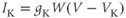
Figure 1.4 Model action potentials. Simulated response to a stimulus pulse, using Hopf parameter set. (a) Sub- and super-threshold voltage responses to the brief current steps in (b). Current amplitudes 1–6 were 150, 460, 480, 490, 500, and 570  A, respectively. Responses 1 and 2 are below, 3 is near, and 4–6 are above firing threshold. (c) Voltages at 1 ms intervals for time course 6 in (a) (colored circles). (d) Model currents, and (e) normalized voltage-dependent conductances underlying response 6. Note the slower kinetics of K-current activation, despite similar
  –
– curves (Figure 1.3b), due to the different kinetic assumptions in the model. (f–i) Trajectories and nullclines (red and green, marking where
  and
and  turn, respectively) in the phase plane. The intersection of the nullclines is a stable equilibrium; the ultimate destination of all trajectories after the brief stimulus pulse. (f) Trajectories corresponding to the voltage time courses in (a). An action potential corresponds to a counterclockwise excursion around the phase plane. (g) Trajectory 6 plotted with the direction field; vectors indicate the direction and rate of movement at any point in the phase plane. (h) Trajectory 6 plotted at 1 ms intervals, as in (c), indicating the speed of motion around the trajectory. The motion slows where V turns on the red nullcline, and where V approaches equilibrium. (i) The flow, represented by trajectories from many initial values in the phase plane. Color indicates speed of motion around the phase plane, from blue (slow) to orange (fast).
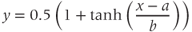
The voltage dependence of steady-state conductance. K-channel activation,  , is assumed to have kinetics and voltage dependence. Both aspects are measured using the voltage clamp, as illustrated in Figure 1.2. In these experiments, the voltage is stepped instantaneously to each of a series of test voltages and held there, while the current reaches a new steady state (Figure 1.2a). Arrival at the steady state is not instantaneous, but defines the kinetics of channel activation, which is itself voltage dependent (Figure 1.2d). We return to the kinetics presently.
The amount of current at the steady state for a test voltage reflects the conformational stability of open states of the K channel; the greater the stability, the more channels open and the greater the conductance. To characterize the voltage dependence of steady-state conductance, the steady-state values of current are first plotted against test voltage to give the current–voltage ( –
– ) plot (Figure 1.2e). Since the measured current is assumed to be the product of driving force and conductance, the current is divided by the driving force to give the conductance–voltage (
 –
– ) plot (Figure 1.2f). To estimate the maximal conductance,
  , the
, the  –
– curve is fit with a Boltzmann function (Figure 1.2f), then
  is given by the maximal value, or upper asymptote, of the Boltzmann curve. The Boltzmann function is then normalized (divided) by
  to yield the proportion,
  , of (activatable) channels that are open at the steady state, as a function of
  .
.
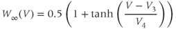
Equations (1.5) and (1.6) define the steady-state open probabilities,  and
and  , for the Ca and K channels, respectively, in our Morris–Lecar model (see Figure 1.3b):
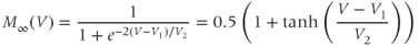
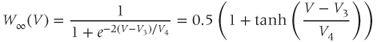
In the next exercises, we will graph  to cement intuition for the role of
  and
and  .
.  is similar. In Exercise 1.2.7, we will confirm that the two different forms of the equations are, indeed, equal. The exercises are written with the online graphing calculator Desmos in mind, but any graphing calculator will do. We choose Desmos because it is fun to work with, and for the ease of setting up sliders to explore the way parameters shape the graph. See Table 1.1 for the values of
  , and
, and  used in later sections of this tutorial.
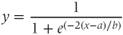
- (1.2.4) Open Desmos in a browser (www.desmos.com). You enter functions in the panel on the left, and watch them appear on the axes on the right. For example, click on the left panel, and type in
 . You should see the familiar exponential function appear. Now click on the next box on the left, and enter
  . Click on the “button” to accept the offer to add a slider for
  . Slide the value of
  (by hand, or by clicking the “play” arrow) and watch your graph shift to the left or right accordingly. Now, try
  . You can add a new slider for
  . What is the effect of sliding
  ? Notice how the old
  slider now works for both the functions. You can temporarily hide a graph by clicking on the colored circle next to its equation, or permanently erase it by clicking on its gray X. There is also an edit button to explore.
- (1.2.5) As we have seen, Desmos uses
 and
and  for variables, and single letters for other parameters. So, to graph
  , you will need to re-write Equation (1.6) with
  playing the role of
  ,
,  playing the role of
  ,
,  playing the role of
  and
and  playing the role of
  . In other words, working with the Boltzmann form of Equation (1.6) first, enter
(being careful with your parentheses!), and accept the sliders for
 and
and  . You should see a typical (normalized)
  –
– curve ranging between 0 and 1, as shown in Figures 1.2f, 1.3b, and 1.3c. Slide
  and
and  to see what role they play in shaping the curve. You can change the limits of the sliders if you like. For example, click on the lower limit of
  and set it to zero, to keep
  positive.
- (1.2.6) Translating back to the language of Equation (1.6), confirm that
 is the half-activation voltage of
  , and
, and  determines the “spread” of
  . As
. As  increases, the spread increases. In other words, as
  increases, the slope at half-activation decreases. In fact, differentiating Equation (1.6) at
  shows that the slope at half-activation is given by
  . Confirm this with Desmos, by graphing the line
  (which has slope
  ) together with Equation (1.7), setting
  , and sliding
  .
.
- (1.2.7) Use Desmos to plot
and confirm that this second form of Equation (1.6) is equivalent to the first. In other words, it has exactly the same graph. This second form is also commonly used, and you will see it in the XPP code provided. If you are unfamiliar with the hyperbolic tangent function,
 , develop your intuition by building up the graph of Equation (1.8) in parts. First graph
  , then
 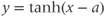 , etc. (Recall that the more familiar
  , and
, and  are defined using a point on the unit circle
  . The hyperbolic functions
  , and
, and  have analogous definitions using a point on the hyperbola
  .)
.)
Voltage-dependent kinetics of voltage gating. Now we return to the kinetics of K-channel gating, governing the rate of approach to the steady state. The channels are trying to reach the steady state for conductance at a particular voltage, but during the process the voltage is typically changing. As a result, the channels are always playing catch-up. Moreover, the rate at which the channels respond to voltage is itself a function of voltage. These kinetics are modeled by the differential equation

Here,  and
and  are both positive, and together define the time scale (or time constant) of K kinetics. The voltage dependence of the time scale is captured by the equation for
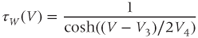
See Figure 1.3c. We will develop intuition for Equations (1.9) and (1.10) in the following exercises. See Table 1.1 for the values of  , and
, and  used in later sections of this tutorial.
- (1.2.8) First let us focus on the
 term in Equation (1.9). It is reminiscent of the
  term in Equation (1.3), and can be analyzed in a similar way. Recall that
  and
and  change over time. So, at a given time
  ,
,  and
and  will have values
  and
and  . What happens if, at time
  ,
,  ? Will
  increase or decrease in the next increment of time? Remember that
  and
and  are both positive. So, if you keep track of the signs, you should find that if
  , then
  , so
, so  is driven down, toward
  .
.
- (1.2.9) What happens if
 ? Explain how the conductance is driven towards steady state in this case, too. As time marches on,
  changes. So the voltage-dependent steady-state conductance,
  , also changes. Thus, the
  term in Equation (1.9) ensures that
  adjusts course accordingly, in its tireless game of catch-up.
- (1.2.10) Now, let us focus on
 to prepare us for understanding its role in Equation (1.9). Use Desmos to graph
  , as shown in Figure 1.3c. Recall that you will need to rewrite the equation for
  with
with  playing the role of
  ,
,  playing the role of
  , and single letters playing the role of
  and
and  . For example, you could graph
with sliders for
 and
and  . Here,
  stands for hyperbolic cosine, the analog of cosine for the hyperbola. If you are unfamiliar with hyperbolic cosine, then build up Equation (1.11) in parts: first graph
  , then
 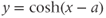 , etc. What role does
  play in the graph of Equation (1.11)? What role does
  play? What is the maximum value of
  ? What is the minimum value? Translating this back to the language of Equation (1.10), you should find that
  reaches a peak value of 1 at
  , and decays down to zero on either side of
  . The rate of decay is governed by
  : the greater the value of
  , the greater the “spread” of
  .
.
- (1.2.11) Recall that
 and
and  are also the shape parameters for
  . Use Desmos to plot the graph of
  on the same axes as your graph of
  (see Figure 1.3c). Use
  to represent
  in both equations, and
  to represent
  . Then, when you slide
  and
and  , you can see their effect on both equations simultaneously. What do you notice?
  and
and  have similar spreads, and
  has its maximum at the half-activation voltage of K conductance.
- (1.2.12) Now, look back at Equation (1.9). Does
 change faster when
  or when
  ? In other words, does
  change faster at half-activation, or far from half-activation? Does that make sense?
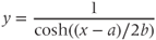
Recapping, Equations (1.9) and (1.10) model the voltage-dependent kinetics of K+ conductance. The time constant  governs the rate at which W catches up with the ever-changing
  . The kinetics are slowest around the half activation voltage where the probabilities of K+ channel opening or closing balance.
Fast calcium kinetics reduce the dimension of the model. Equations similar to (1.9) and (1.10) could be used to model the kinetics of Ca conductance. However, as described in Section 1.1, Morris and Lecar (1981) used the time-scale separation observed between the Ca and K kinetics to reduce the dimension of their model. Instead of including an additional differential equation to follow the very fast approach of Ca conductance to its steady state, they made the assumption that Ca-channel activation occurs immediately, relative to the time scale of K kinetics. In other words, they assume that Ca activation,  , is always “caught-up” to
  . So,
. So,  can be substituted for
  in Equation (1.1), yielding Equation (1.12).
Summarizing. The Morris–Lecar model is given by the system of two coupled nonlinear differential equations

where


The variables, parameters, and parameter values we use are summarized in Table 1.1.
What does the model tell us? Now, we have equations for how  and
and  change! In the rest of the tutorial, we use numerical simulation and graphical analysis to gradually uncover the richness of behavior the minimal mechanisms included in this model cell can exhibit.
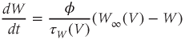
The model is autonomous. Notice that the independent variable, time, does not appear explicitly in the right-hand sides of Equations (1.12)–(1.16). So the system is autonomous, or self-governing, meaning that the rates of change,  and
and  depend only on the state of
  and
and  , and not on when they achieve that state. In Section 1.4, we will see how this autonomous structure is key to the phase-plane approach used throughout the text.
1.3 Opening XPP and triggering an action potential
From here on, you will need a dynamical systems software package to work the interactive exercises. The main tools used in this tutorial are: (1) numerical integration of systems of two and three differential equations, and plotting solutions against time, and (2) phase-plane plots and calculations for systems of two differential equations, including trajectories, direction fields, nullclines, equilibria, limit cycles, and eigenvalues. We will define these terms as we come to them.
There are many good software packages available for simulating differential equations, each with its own strengths and weaknesses. We have written this tutorial to work directly with XPP (also called XPP-Aut), by Bard Ermentrout (2012). We have chosen XPP for several reasons. It is freely available, widely used in the computational neuroendocrine community, and works on many platforms, including Mac, Windows, and Linux machines, all with the same menu system and graphical user interface. We find that it has a good balance of computational power, user friendliness, and modeling freedom. The combination of two-dimensional phase-plane graphics and the capability of simulating higher dimensional models is particularly useful, especially if your goal is to develop more complex models of your own, involving several coupled differential equations. XPP can also simulate many types of differential equation, and a wide range of examples from biology, chemistry, and physics are included with the download.
There are also XPP apps for the iPad and iPhone. The interface is different for these apps, since it makes use of the touch-sensitive screen. Thus, to work this tutorial on an iPad or iPhone, you will need to learn the interface and modify our menu instructions. Similarly, if you prefer a different software package, it should be straightforward to translate the exercises accordingly. For example, PPLANE (MATLAB or Java based, http://math.rice.edu/ dfield) and Berkeley Madonna (www.berkeleymadonna.com) both have user friendly two-dimensional phase-plane graphics. Or you may prefer the independence of Matlab (www.mathworks.com), R (http://www.r-project.org), or Mathematica (http://www.wolfram.com/mathematica). See the online supplementary materials to Ellner and Guckenheimer (2006) for Matlab and R-tutorials, and R-based PPLANE.
Download XPP. At the time of writing, the following steps work to download the Mac, Windows, or Linux versions of XPP.
- Visit Bard Ermentrout’s XPP-Aut page at: http://www.math.pitt.edu/ bard/xpp/xpp.html There isonline documentation, an interactive tutorial, and much more. Read the information for your platform below the DOWNLOAD link, then click on DOWNLOAD.
- Go to Assorted Binaries, then Latest to find the latest binary file for your platform. Mac versions are “dmg” files with “mac” or “osx” in the title somewhere, windows versions are “zip” files with “win” in the title somewhere.
- Download a version for your platform, then open the file install.pdf. Carefully follow the instructions that tell you where to put the files, how to download an “X server,” if necessary, and how to fire up XPP. (If you run into trouble trying to quit XPP, look ahead a couple of pages to the paragraph headed Essential XPP tips.)
ODE files. XPP is a tool for simulating differential equations. It reads the equations from an ODE file written by the user. There is a lot of helpful information about the structure of ODE files, and a wealth of examples, on the XPP website. Example ODE files are also included in the files downloaded with XPP, together with a manual (XPP_doc) and a succinct summary of commands (XPP_sum) in PDF and postscript (ps) formats. XPP was written for applications to neuroscience, and the manual and online tutorial use neural models throughout. It is well worth learning to read and write ODE files, as it gives you control over the nuances of the model, and the freedom to experiment with new models of your own. The components of the ODE file given below will be explained as we work with it in XPP.
Download the ODE file for this tutorial. For the interactive exercises, you will need the file BridgingTutorial-MLecar.ode reproduced below. Electronic copies are available on the website for this volume and from the authors. We recommend downloading an electronic copy, to save yourself the trouble of re-typing it and, more importantly, the possibility of mis-typing. As stated in the XPP manual: “ODE files are ASCII readable files that the XPP parser reads to create machine usable code.” This means that it is important to use a plain text editor for ODE files, because complex editors (such as word) add invisible extra characters to your document that render it unreadable to XPP. Use an editor like Textedit (on a Mac) or NotePad or WordPad (in Windows). Be sure to save the file as plain text such as ASCII, or UTF-8.
# BridgingTutorial–MLecar.ode

# From ‘Bridging Between Experiments and Equations’ by McCobb and Zeeman

# Adapted from online examples by Bard Ermentrout and by Arthur Sherman

# differential equations

dV/dt = (I – gca∗Minf(V)∗(V–Vca) – gk∗W∗(V–Vk) – gl∗(V–Vl))/C

dW/dt = phi∗(Winf(V)–W)/tauW(V)

# functions

Minf(V)=.5∗(1+tanh((V–V1)/V2))

Winf(V)=.5∗(1+tanh((V–V3)/V4))

tauW(V)=1/cosh((V–V3)/(2∗V4))

# default initial conditions


W(0)=0

# default parameters

param I=0,C=20

param Vca=120,Vk=–84,Vl=–60

param gca=4,gk=8,gl=2

param V1=–1.2,V2=18

# uncomment the parameter set of choice

param V3=2,V4=30,phi=.04

# param V3=12,V4=17,phi=.04

# param V3=12,V4=17,phi=.22

# choose a parameter set using ‘(F)ile’ then ‘(G)et par set’ in XPP menu

set hopf   {Vca=120,Vk=–84,Vl=–60,gca=4,gk=8,gl=2,C=20,V1=–1.2,V2=18,V3=2,  V4=30,phi=.04}

set snic    {Vca=120,Vk=–84,Vl=–60,gca=4,gk=8,gl=2,C=20,V1=–1.2,V2=18,V3=12,V4=17,phi=.04}

set homo {Vca=120,Vk=–84,Vl=–60,gca=4,gk=8,gl=2,C=20,V1=–1.2,V2=18,V3=12,V4=17,phi=.22}

# track some currents and conductances

aux Ica = gca∗Minf(V)∗(V–Vca)

aux Ik = gk∗W∗(V–Vk)

aux Il = gl∗(V–Vl)

aux CaCond = gCa∗Minf(V)

aux KCond = gk∗W

aux POpenCa = Minf(V)

aux POpenK = W

# Open XPP with (t,V) voltage–trace window or (V,W) phase–plane window.

@ xp=t,yp=V,xlo=0,xhi=200,ylo=–80,yhi=50

# @ xp=V,yp=W,xlo=–75,xhi=70,ylo=–0.2,yhi=1

# some numerical settings

@ dt=.25,total=200,bounds=10000,maxstore=15000

done
Reading the ODE file. Lines beginning with a # symbol are not read by XPP. They can be used for comments, or to make choices between options by inactivating the unwanted options.
- (1.3.1) Find the differential equations and associated functions in BridgingTutorial-MLecar.ode, and check that they agree with Equations (1.12)–(1.16). The notation is slightly different in XPP, because there are fewer symbols available and no subscripts, but the translation from Equations (1.12)–(1.16) is fairly straightforward. For example, Minf(V), Winf(V), tauW(V), and phi correspond to
 , and
, and  , respectively.
- (1.3.2) Confirm that the parameter values listed in the ODE file agree with those in Table 1.1.
Initial conditions. Recall from Section 1.2 that the differential equations for  and
and  tell us the rate of change of
  and
and  . So, if we know the values of
  and
and  at one initial moment in time, we (or preferably XPP) can numerically predict the future values of
  and
and  by adding on the incremental changes over time. Thus, in order to simulate the time course of
  and
and  , XPP needs initial conditions
  and
and  .
.
- (1.3.3) Find the default initial conditions in the ODE file. What does the initial condition
 tell you about the K channels?
- (1.3.4) The initial membrane voltage is
 . What does this tell you about the Ca channels? Hint: Use the equation for the voltage dependence of Ca-channel gating (Equation (1.14)), with the parameter values from the ODE file (see also Figure 1.3b).
Notice, again, the difference in the way Ca and K channels are treated in the model. The assumption of “instantaneous” kinetics of Ca-channel gating means that the state of the Ca channels at any given time can be deduced directly from the membrane voltage at that time. In particular, the initial state of the Ca channels follows from that of the membrane voltage, as in Exercise 1.3.4. By contrast, the slow response of K channels to changing voltage is tracked by  , which, in turn, depends on their initial state,
  .
.
- (1.3.5) Confirm that the applied current,
 , is set to a default value of zero in the ODE file. In the absence of applied current, and with the default initial conditions, how do you expect this cell to behave?
The rest of the ODE file will be explained as we work with XPP. For more information, see the XPP manual XPP_doc (included with the download and available online (Ermentrout, 2012)).
Opening XPP. Methods for firing up XPP depend on the platform you are using and are described in the file install.pdf included with the download. In all cases, XPP has a console window, and is fired up from the console using an ODE file. On a Mac and Windows computer, the install instructions describe how to set up a shortcut to the XPP console. XPP can be started by dragging an ODE file onto the icon, or into the open console window. On a Linux computer, the install instructions describe how to set up the path and fire up ODE files from the command line (the terminal window then functions as the console). The console reports errors and other useful information.
- (1.3.6) Fire up XPP using the ODE file BridgingTutorial-MLecar.ode. The console will report XPP’s progress on reading the ODE file and, if all is well, an XPP command window will open up. The command window includes a graphics window, a menu down the left-side buttons and a command line along the top, and sliders along the bottom. If the menu and sliders are overlapping, enlarge the window by dragging the bottom right corner. Let us graph the voltage time course of our model cell. Click on the ICs button at the top of the command window. A small window should open, showing the initial condition
 and
and  . Click Go. An unremarkable voltage trace appears on the graph, showing a cell at rest, close to
  . Is this what you expected?
Essential XPP tips. We will use XPP to trigger action potentials, explore and dissect the model behavior, and learn some of the concepts and language of dynamical systems. But first a few essential tips to help give you immediate XPP independence.
- Quitting XPP. There are several ways to quit XPP, none of them quite obvious. In the command window menu, click File then Quit in the submenu, then Yes on the tiny pop-up window. Alternatively, depending on your operating system, you may be able to click Cancel on the console (bottom right), then click Quit in the same place.
- To close a pop-up window, use the close button within the window. The usual way of closing windows (e.g., red button on a mac) may not work.
- The capital letter in the name is the shortcut to each menu item. Within each submenu, there are similar shortcuts, shown in parentheses. For example, typing FQY is a shortcut for quitting XPP. Henceforth, we will show the short cuts in parentheses.
- When you hover over a menu item with the mouse, a brief description is given in the skinny text line along the bottom of the command window.
- Sometimes you need to press the escape key to escape the mode you have put XPP into. For example, the (N)umerics menu is unlike the others: if you enter it, you need to press escape to exit.
- Sometimes XPP needs your input before it can run your command. For example, if you click on (X)i versus t in the menu, it may appear that nothing has happened. In fact, the skinny command line along the top of the command window is asking you which variable you want to plot against time,
 . Enter your choice (e.g.,
  ), then press return.
- So, if XPP seems unresponsive, check to see if it is asking a question in the command line or in a tiny pop-up window (possibly hidden behind other windows). If not, try pressing escape a few times.
- Some menu items only apply to some types of graph. For example, the (D)ir. field/flow menu only works when you are plotting two dependent variables against each other (e.g.,
 versus
  , see Section 1.4). Otherwise, nothing happens when you try it.
- Succinct information about all the main menu and submenu commands is listed in the manual XPP_doc that is downloaded with XPP, and in the Online Documentation on the XPP homepage (Ermentrout, 2012).
- So, if XPP seems unresponsive, check to see if it is asking a question in the command line or in a tiny pop-up window (possibly hidden behind other windows). If not, try pressing escape a few times.
Triggering an action potential. Returning to our model cell, imagine applying a short pulse of positive current, as in a current clamp experiment designed to characterize the cell’s excitability. During the pulse, the membrane voltage will rapidly depolarize (increase), with the amount of depolarization depending on the magnitude and duration of the applied current. The K channels will, in turn, respond to the voltage change, but on a slower time scale. A useful way to think about this, from the modeling point of view, is that the brief stimulus has the effect of resetting the initial values of  and
and  , where the word “initial” now refers to the moment of termination of the stimulus (initiation of the post-stimulus response). In other words, we can think of the initial values of
  and
and  as reflecting the recent history of the cell. In the case of our stimulus pulse, if it is very brief relative to the time scale of the K channels, then
  does not have time to change much during the pulse, so, roughly speaking, only
  is reset. The subsequent effect on
  is seen in the post-stimulus response.
Figure 1.4a shows model voltage responses during and after a range of 2 ms stimulus pulses (amplitudes in Figure 1.4b). Before each pulse, the cell is at rest at  . During the pulse,
  in Equation (1.12), and the voltage rises rapidly. Thus, at the end of the pulse, when
  returns to zero,
  has been “reset.” After the pulse, the cell responds with classic threshold behavior: firing an action potential only if the reset
  is sufficiently high.
In the next exercises, we will use XPP to explore the cell’s post-stimulus response. Instead of modeling the stimulus pulse itself, we will reset the initial value of  directly – as a proxy for the cell’s stimulus history – and plot only the post-stimulus response. In Section 1.4, we will see how this approach lends itself to simultaneously plotting the cell’s response to all possible histories on one graph, called the phase plane. (Note: if you wish to also explore the response during stimulus, an ODE file BridgingTutorial-StimPulse.ode is available on the website for this volume, or from the authors.)
- (1.3.7) Continuing from Exercise 1.3.6, activate the XPP command window by clicking on it. Then click (E)rase to clear the graph. Click the ICs button, if necessary, to re-open the small window showing the initial conditions for
 and
and  . Reset
  to the depolarized value
  (you may need to click once or twice in the box before you can erase or type in it). Leave
  unchanged at 0, and click the Go button. How does the cell respond?
- (1.3.8) The depolarization in the last exercise was evidently not strong enough to trigger an action potential, since the cell returned directly to rest. Try resetting the initial
 to the more depolarized value
  , to represent a stronger stimulus. Now what happens?
- (1.3.9) We saw in the last exercise that the cell fires an action potential if the stimulus is strong enough to reset
 to
to  mV. Experiment with the initial
  to see the decisive, all-or-nothing nature of the response, and reproduce the post stimulus responses of Figure 1.4a. Where is the firing threshold? In other words, approximately what is the smallest value of
  that can trigger an action potential?
Dissecting the action potential. In the next exercises we will plot the post-stimulus time courses of the currents, conductances, and K-channel activation,  , that contribute to the action potential. Then, in Section 1.4, we will analyze the action potential from the phase-plane point of view, as in Figure 1.4f–i.
- (1.3.10) To see the slow K-channel response, let us plot the post-stimulus time course of
 . Click on the command window to activate it, then click on (M)akewindow in the menu, followed by (C)reate in the submenu. A new, small graphics window should open, showing a copy of the most recent
  time course plotted. Notice that the new window does not have its own menu system. Instead, the command window menu applies to whichever graphics window is activated. A tiny black square in the upperleft corner of a graphics window indicates it is active. Activate the new window by clicking in it, and resize it to your taste. Click on (V)iewaxes in the menu, then (2)D in the submenu. Replace
  with
with  for the
  –axis, and, since
  is a proportion, set the
  range from a minimum of 0 to a maximum of 1. Note that you can also set the axis labels:
  for the
  label and
  for the
  label. Then click the OK button. A
  time course should appear in the new graphics window.
- (1.3.11) The
 time course you have plotted corresponds to the initial values of
  and
and  currently displayed in the small ICs window (headed Initial Data). In case you have a confusion of too many plots at this point, you can clear each graphics window by activating it, and then clicking (E)rase in the menu. When both windows are clear, choose an initial condition just above firing threshold (e.g.,
  ), then click the Go button after activating each graphics window in turn.
- (1.3.12) Resize and line up the
 time course graphics window below the original
  time course. Do you see how the K channels are slow, lagging behind the changes in
  ?
?
- (1.3.13) You can also activate all the open graphics windows simultaneously. Click on (M)ake window, followed by (S)imPlot On. Click (E)rase, and notice that both the graphics windows are erased. (Recall that in Exercise 1.3.11 you had to erase one window at a time.) Now click the Go button, to see the
 and
and  time courses plotted simultaneously in the two graphics windows. This can be very convenient, but it does slow XPP down, so remember to turn (S)imPlot off when you do not need it.
- (1.3.14) In our ODE file BridgingTutorial-MLecar.ode, we define several auxiliary quantities (labeled aux in the ODE file), representing different components of the model response. Click on the Equations button at the top of the command window. A small window will pop up listing all the equations from the ODE file. You cannot edit the equations in this small window, but it is useful for reminding you of the names of the auxiliary quantities, and the roles of the parameters. Confirm that the auxiliary equations for the individual currents, conductances, and channel open probabilities agree with those developed in Section 1.2.
- (1.3.15) Now click on the Data button at the top of the command window. A large window will pop up, in which the simulated data for each variable and auxiliary quantity are shown. This data can be exported to a space-delimited dat file using the Write button. Navigate around the data set using the PgDn, PgUp, Right, and Left buttons at the top of the window. Confirm that there are columns for all the auxiliary quantities. Also, confirm that the time increments are 0.25 ms and the total run time is 200 ms. Look back at the ODE file to see how these internal numerical parameters (dt and total) were pre-set, using the @ symbol.
- (1.3.16) Each column in the data viewer can be plotted against time, or the columns can be plotted against each other. One way to plot a time course is by using (V)iewaxes, as in Exercise 1.3.10. A quick alternative is to click (X)i versus t in the menu, then enter the name of the variable or auxiliary quantitity to be plotted in the command line (using the name as it appears in the Eqns and Data windows). When you use (X)i versus t, the axes are automatically scaled to fit the data. The scale can then be adjusted using (V)iewaxes, if desired. Make three new graphics windows (using (M)akewindow, then (C)reate). Line the new windows up underneath each other, and use (X)i versus t to plot the K conductance, the K driving force, and the K current (with initial
 above firing threshold, at
  ).
).
- (1.3.17) Confirm that the graph of K conductance, given by
 , is the same shape as the graph of
  , scaled by
  .
.
- (1.3.18) Why does the K driving force, given by
 , start at 71 mV? Confirm that the graph of K driving force is an upward shift of the graph of
  .
.
- (1.3.19) The K current is given by
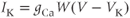 . Describe how the properties of the graph of the K-current result from the properties of the graphs of conductance and driving force. For example, why does the graph of
  start at 0
  A? why does it peak at approximately 250
  A? and why does it drop more suddenly than the graph of K conductance?
- (1.3.20) Let us plot the Ca conductance in the same window as the K conductance. Activate the window, then click on (G)raphic stuff in the menu, followed by (A)dd curve in the submenu, and enter CaCond for the Y-axis (the Z-axis, Color, and Line type can be ignored). Click Ok. Next, use (V)iewaxes to set the
 -axis range from 0 to 4 mS, so both graphs are visible. Confirm that, once again, the Ca channels lead the K channels. (In Figure 1.4e, we plot the normalized conductances, to help compare the kinetics.) Use the equation for Ca conductance in the Equations window, and the initial value of
  , to explain the initial Ca conductance shown on your graph and in the data set.
- (1.3.21) Next, plot the Ca driving force in the same window as the K driving force, using (G)raphic stuff and (A)dd curve again, after activating the appropriate window. At first, nothing new appears on the driving force graph. Explain why not. It might help to look at the data, or the value of
 . Use (V)iewaxes to set the
  -minimum to
  mV. Once again, the driving force is a vertical shift of the graph of
  , but this time
  is shifted down, representing an inward current.
- (1.3.22) Now plot the Ca current on the same graph as the K current, and confirm that it is an inward current, adjusting the axis range as needed (see Figure 1.4d). As before, describe how the properties of the graph of the Ca current result from properties of the graphs of conductance and driving force.
- (1.3.12) Resize and line up the
In silico experiments with XPP. We hope that you are inspired to experiment independently. You could plot the currents and conductances for an initial  just below firing threshold; you could adapt the building blocks developed in the Morris–Lecar model to include more channels or more complex gating properties (see Chapter 2 for inspiration); or you could include calcium dynamics (see Chapters 3 and 4 for inspiration). You could then compare model behaviors to clarify the roles of different channels, gating nuances, and your model assumptions.
Hodgkin–Huxley and Fitzhugh–Nagumo models. The XPP download comes with ODE files for several models of excitability. The Hodgkin–Huxley model (Hodgkin and Huxley, 1952), includes both activation and inactivation, and the kinetics are more realistic, reflecting the number of gating domains required to be in the corresponding state. In the Fitzhugh–Nagumo model (Fitzhugh, 1961; Nagumo et al., 1962), the terms have been abstracted to capture, as simply as possible, the essential geometric features of the nullclines (defined in the next section) that underlie excitability. These and other models recur throughout the text, illustrating the art of letting the biological question determine the level of model complexity to use. They are discussed in most texts on theoretical neuroscience, such as Edelstein-Keshet (2005), Ermentrout and Terman (2010), Fall et al. (2005), Izhikevich (2007), Keener and Sneyd (2008), or Koch (1999).
1.4 Action potentials in the phase plane
In this section, we take a different view of the action potential. We exploit the fact that the Morris–Lecar model has only two dependent variables ( and
and  ) to plot them against each other instead of plotting each against time. Then we see how graphical analysis of the resulting phase plane yields surprisingly many insights into the behavior of the model, through an appeal to our geometricintuition.
- (1.4.1) Let us start afresh. If XPP is not already open, then fire it up with BridgingTutorial-MLecar.ode. If you still have XPP open with lots of graphics windows from the last section, then clean up by clicking (M)akewindow, then (K)ill all (a tiny pop-up window will ask if you are sure). If you have been experimenting with different values for the parameters, then click on (F)ile, followed by (G)et par set and select hopf to restore the default parameters of the Hopf column of Table 1.1. (Look back at the ODE file to see how the parameter set choices available in (F)ile, (G)et par set are coded using the set command.) Set the initial
 and
and  to
to  and
and  , respectively. Plot an action potential in the graphics window, and open the data viewer (Data button in the command window).
Trajectories in the phase plane. The first three columns of simulated data are time, voltage ( ), and K-channel activation (
 ). The familiar voltage trace (or time course) is graphed by plotting the time and voltage columns against each other, but there are many other ways of visualizing the same data. A trajectory in the phase plane is graphed by plotting the
  and
and  columns against each other.
- (1.4.2) Let us plot the trajectory corresponding to the action potential in Exercise 1.4.1. Make a new window ((M)akewindow, (C)reate), and use (V)iewaxes, (2)D to choose
 for the
  -axis and
  for the
  -axis, setting the Xlabel and Ylabel accordingly. Set
  to range from
  to 60, and
  to range from
  to 0.6. (Note that channel activation cannot, in reality, be negative. Our reason for including the negative range is to make it easier to see what’s going on when
  ).
).
- (1.4.3) At first glance the trajectory does not look much like an action potential. We will examine it more closely, to recognize the familiar components of excitability embedded within it. The first row in the data viewer corresponds to time 0 ms, so
 mV and
  (the initial conditions we chose in Exercise 1.4.1). Locate the corresponding point
  in the phase plane. This is where the trajectory starts.
- (1.4.4) Each subsequent row in the data viewer represents a small step forward in time, and each corresponding
 point is plotted in the phase plane. The resulting curve is the trajectory with initial condition
  . Use the Down button at the top of the data window to confirm that when
  ms,
ms,  is approximately 8.3 mV and
  is approximately 0.13. Locate the corresponding point on the trajectory.
- (1.4.5) As time progresses, the cell continues around the trajectory. What is the peak voltage reached? When does it peak? What proportion of K channels are open when it peaks? Which of these questions can be answered using: (i) the phase plane? (ii) the voltage trace? (iii) the data viewer? Confirm that they give the same answers, where applicable.
Translating between a time course and the phase plane. It takes some practice to relate the “vertical” voltage axis of the time course to the “horizontal” voltage axis of the phase plane. Figure 1.4c and h illustrates how motion around the phase-plane trajectory corresponds to the action potential time course. The dots mark equal time intervals of 1 ms. There is no time axis in the phase plane. Instead, the progression of time is captured by progression around the trajectory. (The solid red and green curves in the phase plane are the nullclines, defined later in this section.) During the rapid depolarization and hyperpolarization segments of the spike in the voltage trace, voltage ( ) is changing much faster than K-channel activation (
 ), thus yielding the rapid, roughly “horizontal” segments of the trajectory in the phase plane. Around the peak of the voltage trace, and during hyperpolarization, the voltage changes more slowly, so the K channels have time to open (close, respectively), and the motion around the phase plane has more “vertical” component. As voltage gradually returns to rest,
  also stabilizes, and the trajectory approaches an equilibrium point in the phase plane. In summary, the explosive action potential characteristic of excitability corresponds to a large counterclockwise excursion around the phase plane before returning to equilibrium.
- (1.4.6) Figure 1.4f shows six trajectories in the same phase plane, corresponding to the post-stimulus components of the six voltage traces in Figure 1.4a. Each trajectory has a different initial condition, as set by the pulsatile stimuli shown in Figure 1.4b. Which of the trajectories has initial condition
 ? And which has the initial condition
 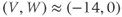 ? Explain how you know.
- (1.4.7) More generally, any point
 in the phase plane can be used as initial data for the model. XPP allows you to select initial points with the mouse as follows. Activate the phase plane, then click (I)nitialconds in the side menu of the command window (not the ICs window we have used so far.) Select m(I)ce in the submenu. A tiny pop-up window appears with instructions. Experiment with initial points all over the phase plane. Press the escape key to exit this mode of choosing initial points when you are ready. Recall that we can view the initial condition of our model cell as reflecting its recent history. What history could lead to each initial point you chose? Some of them are more physiologically meaningful than others. Do the corresponding trajectories make sense? Remember you can turn (S)implot on (in the (M)akewindow menu), if you would like to see the corresponding voltage traces simultaneously, and you can click (E)rase, for a fresh start.
- (1.4.8) The family of all trajectories is called the flow of the system. Erase everything, and turn Simplot off (it is off if the menu toggle offers to turn it on). To plot a representative sample of the flow, called a phase portrait, activate the phase plane and click on (D)ir. field/flow, followed by (F)low. Press return to accept the suggestion, in the command line, of a
 grid of initial points, and watch the beautifully flowing dynamics emerge. Try experimenting with different sized grids.
The phase portrait shows the full range of behavior. A powerful feature of the phase plane is that it shows the cell’s response to all possible histories, all at once. It gives immediate intuition for the full range of responses this cell can exhibit. The cell can fire at most one action potential and all trajectories eventually settle at the same rest point. The “all-or-nothing” quality of the response is captured by the very thin threshold region dividing trajectories that take the large, counterclockwise excursion from those that return directly to rest, and we see that there is, in fact, some variability in the amplitude of the excursion (or spike). In later sections, we will explore how a sustained stimulus expands this range of behaviors.
Trajectories never cross. Another powerful feature of the phase plane is that trajectories may flow toward each other, but they never cross. This has profound consequences for two-dimensional systems, because it means each trajectory imposes a spatial barrier to all the others, trapping them in different regions of the phase plane. This fundamental geometric fact that one-dimensional curves form barriers in a two-dimensional plane explains why geometric phase-plane analysis is so powerful, and can lead to qualitative predictions with relative ease. To understand why trajectories cannot cross each other, it is helpful to relate our model equations (1.12)–(1.16) directly to the phase plane:
- (1.4.9) Equations (1.12) and (1.13) govern the time course of
 and
and  for our model cell. Using
 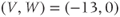 , and the parameter values in the Hopf column of Table 1.1, do the calculations to confirm that
  and
and  . Thus, the rate of change of
  is
is  mV/ms, and the rate of change of
  is
is  ms−1.
ms−1.
- (1.4.10) At the rates given in Exercise 1.4.9, in 1 ms,
 would increase by 0.95 mV to
  mV and
  would increase from 0 to 0.01. Carefully sketch, on paper, the arrow, or vector, pointing from the initial point
  to the new point
 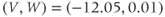 . Your vector has components
 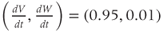 , and shows the instantaneous direction of motion that a trajectory passing through the point
  must follow. Use XPP to plot the trajectory with initial condition
  , and confirm your direction vector agrees with the direction of the trajectory at
  . (You may need to adjust the scale on the axes to make the comparison.)
- (1.4.11) The direction field of the system consists of the vectors
 representing the direction of motion all over the phase plane. To plot a representative sample of direction vectors, as shown in Figure 1.4g, activate the phase plane and click on (D)ir. field/flow, followed by (D)irect Field, and press return to accept a
  grid of initial points.
- (1.4.12) Revisit Exercises 1.4.9 and 1.4.10 to confirm that the different lengths of the direction vectors indicate the relative speed of motion around the phase plane. (In contrast, (D)ir. field/flow, followed by (S)caled Dir. Fld, shows all the direction vectors scaled to the same length.)
- (1.4.13) Choose initial conditions (using (I)nitialconds, m(I)ce) to superimpose individual trajectories on the direction field (as shown in Figure 1.4g). Alternatively, you can superimpose the flow (as demonstrated in Exercise 1.4.8). Notice that trajectories always travel in the direction of motion dictated by the direction field. This is not a coincidence. This is what it means for trajectories to be solutions of the system of differential equations (1.12) and (1.13). Now, it is clear why trajectories cannot cross each other. They have to follow the direction field. And the direction field cannot point in two different directions at once.
Autonomous systems. This is a good moment to emphasize that the argument we just used, and the entire phase-plane viewpoint, depends on the fact that our model equations (1.12)–(1.16) are autonomous. Recall from Section 1.2 that this means that the independent variable, time, does not appear explicitly on the right-hand side of the equations. So the direction vector through a given point  does not change over time, and can only point in one direction.
Nullclines. Recapping, we have seen that the range of behaviors our model cell can exhibit is predicted by the flow in the phase plane. The flow, in turn, follows the direction field, which is given by the differential equations. We now introduce the nullclines of the system, which give a quick guide to how the direction field is organized.
- (1.4.14) Erase everything and plot the flow with a
 grid (e, d, f, then return, via shortcut keys). Now plot the nullclines by clicking on (N)ullcline, and then (N)ew. (Recall that you can hover over each menu item for a description along the bottom of the command window, if you wish). There are two nullclines, one red and one green, as in Figure 1.4f–i. How can you tell the nullclines are not trajectories? (Hint: trajectories do not cross.)
- (1.4.15) So what are the nullclines? Let us uncover their meaning from the XPP plot, starting with the red nullcline. What do you notice about the direction of the trajectories as they cross the red nullcline? And what would that correspond to on the associated voltage traces? It may help to make your graphics window huge, and redraw everything.
Nullclines mark turning points. The trajectories always “turn back” on themselves at the red nullcline. Below the red nullcline, trajectories flow to the right (as well as flowing “up” or “down” the phase plane). At the nullcline they turn, so that above the red nullcline trajectories flow to the left. Those that reach the red nullcline again, at the far left of the graph, turn again, flowing gently rightwards towards the equilibrium point. This observation yields the definition. Rightward and leftward flow in phase space correspond to increase and decrease in voltage, respectively. Thus, the red nullcline marks the points in the phase plane where the voltage turns. In more biological words it marks the peaks and troughs of the corresponding voltage trace. In more mathematical words, it marks the points where the graph of  against
  has a maximum or minimum (or inflection point). So the red nullcline marks the points where
  , and is, therefore, called the V-nullcline.
- (1.4.16) Recall from Exercises 1.4.9 to 1.4.11 that the direction field consists of the vectors
 evaluated at each point. Use this to explain as to why the flow is parallel to the
  axis as it crosses the
  -nullcline. (Hint:
  on the V-nullcline.)
- (1.4.17) The (green)
 -nullcline is defined analogously. Use your XPP plot to confirm that
  on the green nullcline. In other words, flow across the
  -nullcline is parallel to the
  axis, and the nullcline marks the points where trajectories turn from increasing
  (K channels opening) to decreasing
  (K channels closing), or vice versa.
 - (1.4.17) The (green)
Nullclines organize the direction field. Presently, we will examine how the shape of the nullclines is derived from the model equations. First, we will explore how the nullclines mark equilibria and organize the direction field, giving a rough, but immediate, guide to the dynamics of the system.
- (1.4.18) Erase everything, and plot the direction field with a
 grid (e, d, d then return). If the nullclines do not redraw automatically, plot them again (n, n). The nullclines divide the phase plane into regions. Confirm that, in each region, the direction vectors all point in roughly the same direction or quadrant (e.g. upward and rightward, or upward and leftward, etc.) Explain why. (Hint: nullclines mark turning points).
- (1.4.19) What happens at the point where the two nullclines meet? Let us call it point
 . Try choosing initial conditions exactly at
  (using i,i). Nothing appears to happen. Why? (Remember to escape from i,i mode when you are done.)
Equilibria lie at the intersection of nullclines. The point  lies on both nullclines, so both
  and
and  at
at  . Thus, from initial point
  , there is no change in
  or
or  , the direction vector reduces to
  , and the trajectory is fixed at
  for all time. We call
  an equilibrium or fixed point of the system. By the same argument, every intersection of the two nullclines yields an equilibrium, and every equilibrium lies at an intersection of the nullclines.
- (1.4.20) Try choosing initial conditions close to
 (using i,i again). Confirm that trajectories from all nearby initial conditions converge to
  . In other words,
  represents rest, where our model cell stabilizes. Thus, we call
  a stable equilibrium or attractor.
Stable versus unstable equilibria. We classify the stability of an equilibrium according to the behavior of the system near the equilibrium. If nearby initial conditions are all attracted to an equilibrium, it is stable. If they are generally repelled from the equilibrium, it is unstable. The very fact that systems settle down at stable equilibria makes them easy to observe in nature and experimentally, while unstable equilibria are much more difficult to observe. In the next sections, we will see how stable and unstable phenomena interact to shape both the transient and long-term dynamics of the system.
What determines the shape of the nullclines? We will use a combination of algebra and XPP experiments to develop intuition for the nullcline shape. Algebraically, each nullcline can be viewed as the graph of some equation of the form  in the
  –
– phase plane. We will find these equations, to see which model parameters influence each nullcline.
 –nullcline. We will start with the
  nullcline, because the algebra is simpler. Recall that the
  component of direction vectors in the phase plane is given by Equation (1.13)
Related posts:
 Modeling Endocrine Cell Network Topology
Stay updated, free articles. Join our Telegram channel

Full access? Get Clinical Tree


