Introduction

Biostatistics and bioinformatics deal with quantitative information in medical research. Both disciplines involve data analysis and experimental design. No sharp delineation exists between the two, but bioinformatics tends to deal with data in many dimensions, so-called “big data,” such as in genomics. Both disciplines are concerned with making inferences and thus use similar tools and methodology. Relative to bioinformatics, biostatistics is an old discipline. However, the biostatistical aspects of this chapter are modern and describe responses to challenges arising from recent advances in cancer biology. The goal of the chapter is to convey an understanding of new approaches in clinical trial design and analysis.

Biostatistics Applied to Cancer Research

The modern era of cancer therapy raises major issues regarding statistical inference and study design. First, as biomarkers become available, they divide cancers into ever smaller subsets, with unique biomarker-defined combinations of targeted therapies for each subset. Soon every patient with cancer will have an orphan disease. A related issue is the ever-increasing cost of drug development and the consequent cost of delivering care to persons with cancer. Unless we modify our approaches to cancer research, we will not be able to afford the therapies we develop, and innovation will cease.

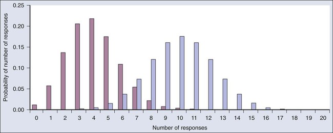
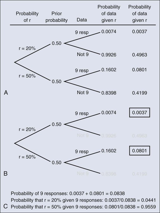
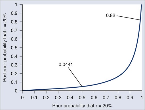
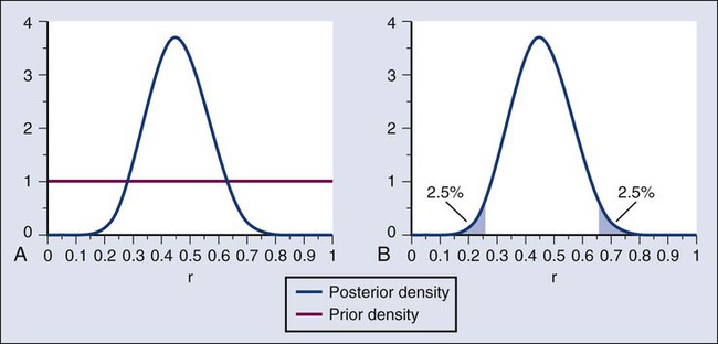
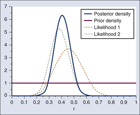
Biostatistical philosophy is critical in understanding the state of cancer research today and where it is heading. Biostatistics has had an immense impact on the level of science in cancer research, especially in designing and conducting clinical trials. However, as we make progress in developing better cancer therapeutics, patients’ prognoses improve, and clinical trials get larger because they are event driven. The irony is that despite the development of cancer in increasing numbers of persons in the world, fewer clinical investigations are possible because of limited resources, and fewer drugs can be developed despite the burgeoning number of potential anticancer drugs. False-positive and false-negative conclusions are well known, but the most frustrating problem in the modern era may be the number of “false neutrals”—drugs and therapeutic strategies that are never investigated because of insufficient resources.

The history of biostatistics is dominated by the so-called frequentist approach. An alternative approach, the Bayesian approach, was largely ignored as biostatistics developed into a discipline. In the frequentist approach, probabilities are defined as long-run proportions. The focus is on the final results of a clinical trial, say, with the unit of inference being the entire trial rather than, for example, a patient within the trial.

For reasons discussed in this chapter, much interest has recently been expressed in the Bayesian approach to statistics. In the first half of the twentieth century there were few Bayesian biostatisticians, and few biostatisticians knew what it meant to be Bayesian.

The Bayesian approach predates the frequentist approach. Thomas Bayes developed his treatise on inverse probabilities in the 1750s, and it was published posthumously in 1763 as “An Essay towards Solving a Problem in the Doctrine of Chances.” Laplace picked up the Bayesian thread in the first quarter of the nineteenth century with the publication of Théorie Analytique des Probabilités. The works of both scientists were important and had the potential to quantify uncertainty in medicine. Indeed, Laplace’s work influenced Pierre Louis in France in the second quarter of the nineteenth century as Louis developed his “numerical method.” Louis’ method involved simple tabulations of outcomes, an approach that was largely rejected by the medical establishment of the time. The stumbling block was not how to draw inferences from data tabulations.¹ Rather, the counter argument and the prevailing medical attitude of the time was that each patient was unique and the patient’s doctor was uniquely suited to determine diagnosis and treatment. Vestiges of this attitude survive today.

In the two hundred years after Bayes, the discipline of statistics was influenced by probability theory, and in particular, games of chance, dating to the early 1700s.4–4 This view focused on probability distributions of outcomes of experiments, assuming a particular value of a parameter. A simple example is the binomial distribution. This distribution gives the probabilities of outcomes of a specified number of tosses of a coin with known probability of heads, which is the distribution’s parameter. The binomial distribution continues to be important today. For example, it is used in designing cancer clinical trials in which the end point is dichotomous (tumor response or not, say) and assuming a predetermined sample size.

Clinical Trials

A clinical trial is an experiment involving human subjects with the goal of evaluating one or more treatments for a disease or condition. A randomized clinical trial (RCT) compares two or more treatments in which treatment assignment is determined by chance, such as by rolling a die or tossing a coin.

The traditional statistical approach is to consider two possible values of the unknown parameters, such as the tumor response rate r. For one value of r the treatment has no useful benefit, the so-called null hypothesis. The alternative hypothesis is a value of r that is clinically important in the sense of meriting future development.

Consider a single-arm clinical trial with the objective of evaluating r. The null value of r is taken to be 20%. The alternative value is r = 50%. The trial consists of treating n = 20 patients. The exact number of responses is not known in advance, but it is known to be either 0 or 1 or 2 on up to 20. The relevant probability distribution of the outcome is binomial, with one distribution for r = 20% and a second distribution for r = 50%. These distributions are shown in Figure 19-1, with red bars for r = 20% and blue bars for r = 50%. More generally, there is a different binomial distribution for each possible value of r.

Both the frequentist and Bayesian approaches to clinical trial design and analysis utilize distributions such as those shown in Figure 19-1, but they use them differently.

Frequentist Approach

The frequentist approach to inference is based on error rates. A type I error is rejecting a null hypothesis when it is true, and a type II error is accepting the null hypothesis when it is false, in which case the alternative hypothesis is assumed to be true. It seems reasonable to reject the null, r = 20% (red bars in Fig. 19-1) in favor of the alternative, r = 50% (blue bars in Fig. 19-1) if the number of responses is sufficiently large. Candidate values of “large” might reasonably be where the red and blue bars in Figure 19-1 start to overlap, perhaps nine or greater, eight or greater, seven or greater, or six or greater.

The type I error rates for these rejection rules are the respective sums of the heights of the red bars in Figure 19-1. For example, when the cut point is 9, the type I error rate is the sum of the heights of the red bars for 9, 10, 11, etc., which is 0.007387 + 0.002031 + 0.000462 + … = 0.0100. When the cut points are 8, 7, and 6, the respective type I error rates are 0.0321, 0.0867, and 0.1958. One convention is to define the cut point so that the type I error rate is no greater than 0.05. The largest of the candidate type I error rates that is less than 0.05 is 0.0321, the test that rejects the null hypothesis if there are eight or more responses. The type II error rate is calculated from the blue bars in Figure 19-1, where the alternative hypothesis is assumed to be true. The sum of the heights of the blue bars for 0 up to 7 responses is 0.1316. Convention is to consider the complementary quantity and call it “statistical power:” 0.8684, which rounds off to 87%.

The distinction between “rate” and “probability” in the aforementioned description is important, and failing to discriminate these terms has led to much confusion in medical research.⁵ The “type I error rate” is a probability only when assuming that the null hypothesis is true. Probabilities of events requiring the truth of the null hypothesis are not available in the frequentist approach, and indeed this is a principal contrast with the Bayesian approach (described later).

Suppose the trial is conducted and 9 of 20 patients respond. One concludes that the null, r = 20%, is rejected because 9 is greater than the predetermined cut point of 8. However, the results are more convincing than had the result been exactly 8. Such reasoning led to the convention of reporting a P value, an “observed type I error rate.” This is the type I error rate had the predetermined cut point been set to the observed number. Thus the P value is .0100, as calculated earlier.

Values of r other than 20% and 50% are possible. The standard frequentist approach to representing the range of possibilities is to provide a confidence interval, which is the set of values of r that would not be rejected as null hypotheses based on the data actually observed: 9 responses out of 20 patients (or 45%). For these data, the values of r that would be rejected are those less than 26%. Because very large values of r are also inconsistent with the observed rate of 45%, it is conventional to also exclude large values from the confidence interval. Assuming type I error rates of 5% for both small and large values of r, the resulting confidence interval is from about 26% to 61%, which is a 90% confidence interval in the sense that 5% is excluded on both sides. Excluding only 2.5% on each side provides a 95% confidence interval: 23% to 64%. Ninety-five percent confidence intervals are commonly used and are always somewhat wider than 90% confidence intervals.

Bayesian Approach

A major difference between the Bayesian and frequentist approaches is the use of probability distributions to represent unknown values. In the frequentist approach, probabilities apply only for “data.” Parameters that index data distributions (such as r in the aforementioned example) are unknown but are fixed and thus are not subject to probability statements. In the Bayesian approach, all unknowns, including parameters, have probability distributions.

In the example in which 20 patients yielded 9 responses, suppose that r is assumed to be either 20% or 50%. The Bayesian conclusion is the probability of r = 50%, given the final results. (This is one minus the probability of r = 20% under the assumption that these are the only two possible values of r.) The calculation uses Bayes’ rule. The method is the same as when finding the positive predictive value of a test as it relates to the condition’s prevalence and the test’s sensitivity and specificity. Bayes’ rule is also called the “rule of inverse probabilities” because it relates the probability of some event A given that event B has occurred with the probability of event B given that event A has occurred.

The calculation is intuitive when viewed as a tree diagram, as in Figure 19-2. Figure 19-2, A, shows the full set of probabilities. The first branching shows the two possible parameters, r = 20% and r = 50%. The probabilities shown in the figure, 0.50 for both, will be discussed later. The data are shown in the next branching, with the observed data, nine responses (nine resp) on one branch and all other data on the other. The probability of the data given r, which statisticians call the likelihood of r, is the height of the bar in Figure 19-1 corresponding to nine responses, the red bar for r = 20%, and the blue bar for r = 50%. The rightmost column in Figure 19-2, A, gives the probability of both the data and r along the branch in question. For example, the probability of r = 20% and “nine resp” is 0.50 multiplied by 0.0074.

The probability of r = 20% given the experimental results depends on the probability of r = 20% without any condition, its so-called prior probability. The analog in finding the positive predictive value of a diagnostic test is the prevalence of the condition or disease in question. Prior probability depends on other evidence that may be available from previous studies of the same therapy in the same disease, or related therapies in the same disease or different diseases. Assessment may differ depending on the person making the assessment. Subjectivity is present in all of science; the Bayesian approach has the advantage of making subjectivity explicit and open.⁶

When the prior probability equals 0.50, as assumed in Figure 19-2, the posterior probability of r = 20% is 0.0441. Obviously, this is different from the frequentist P value of 0.0100 calculated earlier. Posterior probabilities and P values have very different interpretations. The P value is the probability of the actual observation, 9 responses, plus that of 10, 11, etc. responses, assuming the null distribution (the red bars in Fig. 19-1). The posterior probability conditions on the actual observation of nine responses and is the probability of the null hypothesis—that the red bars are in fact correct—but assuming that the true response rate is a priori equally likely to be 20% and 50%.

P values are not intuitive in that they condition on a hypothesis that seems unlikely to be true in view of the results (the null hypothesis) and because they depend on probabilities of possible occurrences that were not observed. For example, if there are two candidate null distributions with the same probability of the actual observation, the one with the smaller “tail” of unobserved values will have a smaller P value. Because they are counterintuitive, misinterpretations of P values abound. People usually convert a P value into something they understand but which is wrong, and the misinterpretation usually has a Bayesian ring to it; for example, “The P value is the probability that the results could have occurred by chance alone.” An objection to Bayesian inferences is that they are specific to assumed prior probabilities. A sensible type of report that addresses this concern is the following: “If your prior probability is this, then your posterior probability is that.”

As an example of such a report, Figure 19-3 shows the relationship between the prior and posterior probabilities. The figure indicates that the posterior probability is moderately sensitive to the prior. Someone whose prior probability of r = 20% is 0 or 1 will not be swayed by the data. However, as Figure 19-3 indicates, the conclusion that r = 20% has low probability is robust over a broad range of prior probabilities. A conclusion that r = 20% has moderate to high probability is possible only for someone who was convinced that r = 20% in advance of the trial.

In the example, r was assumed to be either 20% or 50%. It would be unusual to be certain that r is one of two values and that no other values are possible. A more realistic example would be to allow r to have any value between 0 and 1 but to associate weights with different values depending on the degree to which the available evidence supports those values. In such a case, prior probabilities can be represented with a histogram (or density). A common assumption is one that reflects no prior information that any particular interval of values of r is more probable than any other interval of the same width. The corresponding density is flat over the entire interval from 0 to 1 and is shown in red in Figure 19-4, A.

The probability of the observed results (9 responses and 11 nonresponses) for a given r is proportional to r⁹(1-r)¹¹, with the likelihood of r based on the observed results. The prior density is updated by multiplying it by the likelihood. Because the prior density is constant, this multiplication preserves the shape of the likelihood. Thus the posterior density equals just the likelihood itself, shown in green in Figure 19-4, A.

The Bayesian analog of the frequentist confidence interval is called a probability interval or a credibility interval. A 95% credibility interval is shown in Figure 19-4, B: r = 26% to 66%. It is similar to but different from the 95% confidence interval discussed earlier: 23% to 64%. Confidence intervals and credibility intervals calculated from flat prior densities tend to be similar, and indeed they agree in most circumstances when the sample size is large. However, their interpretations differ. A credible interval has a particular probability that the parameter lies in the interval. Statements involving probability or chance or likelihood cannot be made for confidence intervals.

Any interval is an inadequate summary of a posterior density. For example, although r = 45% and r = 65% are both in the 95% credibility interval in the aforementioned example (Fig. 19-4), the posterior density shows the former to be five times as probable as the latter.

A characteristic of the Bayesian approach is the synthesis of evidence. The prior density incorporates what is known about the parameter or parameters in question. For example, suppose another trial is conducted under the same circumstances as the aforementioned example trial, and suppose the second trial yields 15 responses among 40 patients. Figure 19-5 shows the prior density and the likelihoods from the first and second trials. Multiplying likelihood number 1 by the prior density gives the posterior density, as shown in Figure 19-4. This now serves as the prior density for the next trial. Multiplying that density by likelihood number 2 gives the posterior density based on the data from both trials, and is shown in Figure 19-5. The order of observation is not important. Updating first on the basis of the second trial gives the same result. Indeed, multiplying the prior density, likelihood number 1, and likelihood number 2 in Figure 19-5 together gives the posterior density shown in the figure.

The calculations of Figure 19-5 assume that r is the same in both trials. This assumption may not be correct. Different trials may well have different response rates, say r₁ and r₂. In the Bayesian approach, these two parameters have a joint prior density. One way to incorporate into the prior distribution the possibility of correlated r₁ and r₂ is to use a hierarchical model in which r₁ and r₂ are regarded to be sampled from a probability density that is unknown, and therefore this density itself has a probability distribution. More generally there may be multiple sources of information that are correlated and multiple parameters that have an unknown probability distribution. A hierarchical model allows for borrowing strength across the various sources depending in part on the similarity of the results.^9–9

A rather different application of Bayesian hierarchical models, called a “tumor agnostic,” is destined to become important in cancer clinical trials. Consider an agent targeted at a particular mutation. There may be subsets of patients that harbor this mutation across a broad range of tumor types. The mutation may be rare in some or all tumor types. Mustering a compelling clinical trial in any given tumor type may be impossible. Instead, one might conduct a single trial across ten tumor types, say, regarding response rates r₁, r₂, …, r₁₀ as a sample from a population. The population distribution may be homogeneous, in which case there is substantial “borrowing of strength” across the tumor types. This may enable a claim of effectiveness in tumor types that, when left to stand alone, would have wide credibility intervals because of their small sample sizes. On the other hand, if the population of response rates is heterogeneous, then the observed response rates will be highly variable, and borrowing will occur mainly across neighboring tumor types.

We next apply the Bayesian perspective in two important directions that are the focus of attention in modern cancer research.

Adaptive Designs of Clinical Trials

Randomization was introduced into scientific experimentation by R.A. Fisher in the 1920s and 1930s and applied to clinical trials by A.B. Hill in the 1940s.¹⁰ Hill’s goal was to minimize treatment assignment bias, and his approach changed medicine in a fundamentally important way. The RCT is now the gold standard of medical research. A mark of its impact is that the RCT has changed little during the past 65 years, except that RCTs have gotten bigger. Traditional RCTs are simple in design and address a small number of questions, usually only one. However, progress is slow, not because of randomization but because of limitations of traditional RCTs. Trial sample sizes are prespecified. Trial results sometimes make clear that the answer was present well before the results became known. The only adaptations considered in most modern RCTs are interim analyses with the goal of stopping the trial on the basis of early evidence of efficacy or for safety concerns. There are usually few interim analyses, and stopping rules are conservative. As a consequence, few trials stop early.

In traditional RCTs, randomization proportions are fixed throughout. The possibility that the accumulating data in the trial can influence randomization probabilities or other aspects of a trial’s course may affect the trial’s performance characteristics, including its type I error rate and statistical power. Moreover, these effects may be difficult to analyze using traditional mathematics. However, modern computers and software make traditional mathematics unnecessary. Any prospective trial design, however complicated, can be simulated. A prospective trial design is an automaton. At any time during the trial and based on the information available from trial participants, the next patient is assigned a particular therapy, possibly based on an adaptive randomization scheme. Any trial that has a prospective design can be simulated. Virtual patients can be generated with their outcomes depending on assumed parameter values and treatment assignment according to the prospective design. Replicating the trial 10,000 times, say, gives a firm handle on the trial conclusion for the parameter values assumed in the simulation.

Consider a simple case, a variant of the earlier example in which the response rate r was assumed to be either 20% or 50%. Set the maximum number of patients in the trial to 20. Stop the trial with a claim favoring the alternative hypothesis r = 50% whenever the probability of r = 50% versus r = 20% is at least 95% (and therefore the probability of r = 20% is less than 5%).

As a check that the reader is following this description: the binomial distribution assumed earlier is no longer relevant, even if the final sample size happens to be 20. Consider an extreme case. The binomial distribution gives positive probability to 20 responses regardless of the value of r (unless r = 0). However, the adaptive design would have stopped long before getting to 20 patients when every patient represented a response to the treatment—in fact, the trial would have stopped after four responses in four patients.

It happens that for this simple adaptive design it is possible to find its operating characteristics algebraically, but the calculations are tedious. In more complicated circumstances, algebraic calculations may not be possible and simulations are necessary.

Simulations are easy to describe. To address r = 50%, start with a fair coin, one with probability of heads equal to 50% and interpret “heads” to mean response. Whenever a patient is accrued to the trial, toss the coin, observe the result, and update the probability that r = 50% on the basis of the tosses thus far. Stop the trial if this probability is greater than 95% and make a mark so indicating. If the number of tosses reaches 20 without having made a mark, then stop the trial because you have hit the maximal sample size. When the trial stops, make a note of the total number of tosses, say n, in the trial. Repeat the trial a total of 10,000 times. Count the number of marks and divide by 10,000. This is the estimated power of the study assuming r = 50%. Tabulate the 10,000 values of n to give an estimate of the distribution of the final sample size under the alternative hypothesis. (You should have a mark for every trial with n < 20 and also for some trials with n = 20.)

To find the type I error rate, repeat the aforementioned process with another set of 10,000 iterations generated using a device that has probability of heads equal to 20%. (An example device is a regular 20-sided die with “heads” labeled on four of the sides.) The proportion of marks is the estimated type I error rate. The tabulated values of n are the estimated distribution of the final sample size under the null hypothesis.

Tossing a coin perhaps a hundred thousand times will take a while, especially because you will have to keep track of which trial you are in and whether you have achieved the stopping boundary for that trial. The good news is that a simple program running on a modern desktop computer can simulate 10,000 trials in a few seconds. The computer does all the work. Moreover, an additional few seconds gives you another 10,000 simulated trials assuming another value of r by simply changing the value of r in the program.

Figure 19-6 shows the sample size distribution for 10,000 trials under the assumption that r = 50%. The estimated type II error rate is 0.1987, which is the proportion of these 10,000 trials that reached n = 20 without ever concluding that the posterior probability of r = 50% is at least 95%. The sample size distribution when r = 20% is not shown but is easy to describe: 9702 of the trials (97.02%) went to the maximum sample size of n = 20 without hitting the posterior probability boundary and the other 3% stopped early (at various values of n

Related posts:

Hematopoietic Stem Cell Transplantation Control of the Cell Cycle Melanoma Cancer of the Anal Canal Cancers Arising in the Ovary Eye, Orbit, and Adnexal Structures

Stay updated, free articles. Join our Telegram channel

Join