that is, evolution with time of tumor cell density (c) at each position in the brain = proliferation (ρc) + diffusion (∇.(D∇c)).
The direct problem consists to compute this equation numerically, on a digital brain template, for given values of ρ and D. The results of the simulations give the evolution over time of maps of tumor cell density (see Fig. 31.1). The template is usually a generic atlas. Over the past decade, advances has been made in integrating a more precise anatomy in this atlas (see Fig. 31.1): whereas the very first templates were built from a 2D CT scan [2, 3], just outlining the brain surface and the ventricles, more recent works are based on 3D-MRI atlases (on which CSF, white and grey matter segmentations are performed [4]), eventually including detailed white matter architecture via DTI sequences [5, 6]. In that case, the D in the equation should read as a tensor of cell diffusion, which can be built from the tensor of water diffusion, introducing a factor r of anisotropy increase between the two tensors. Diffusion images from an individual healthy volunteer are used [5, 6], but future studies could rely on a tractographic atlas or incorporate own patient DTI MRI. Whatever the elected template, it is of utmost importance that an expert validates its anatomical accuracy. For example, as explained in [6], a wrong segmentation of the subarachnoidal spaces can create artificial bridges of grey matter, especially between the frontal and temporal operculum, leading to unrealistic growth patterns in the simulations. In an effort to correct such inaccuracies, an expert-validated mask of subarachnoidal spaces has been recently built, that greatly improves the veracity of the virtual growth patterns [7].


Fig. 31.1
Advances over a decade in the anatomical accuracy of the simulations. The very first templates in 1995 were built from a 2D CT scan [2, 3], just outlining the brain surface and the ventricles. More recent works in 2000 were based on 3D-MRI atlases (on which CSF, white and grey matter segmentations were performed [4]). Finally, in 2005 detailed white matter architecture via DTI sequences was eventually included [6]
31.2.2 The Visibility Threshold Hypothesis
The tumoral cell density, which is the variable in the proliferation-diffusion model, is not directly measured on MRI. One has to make the reasonable and simple assumption that the tumor is visible on flair MRI at the condition that tumor cell density is above a given value (visibility threshold). Hence the link between simulated and real tumors relies on the comparison between the thresholded isocontour on cell density maps and the effective contours of the tumor on MRI. Unfortunately, there are very few datas in the literature about the value of this visibility threshold. Only one study correlating histological analysis with hypodensity on CT suggested a value of 8000 cells/mm3 [1]. Actually, current studies on this topic suggest that the MRI flair hypersignal is not only dependent on the cell density but is also correlated to the intra- and extra-cellular water content [8]. Hence, it should kept in mind that the visibility threshold hypothesis is a strong approximation, and that most of the following results will be based on this assumption.
31.2.3 Model-Based Assessment of Tumor Dynamics
To go a step further towards clinical application, one needs to solve the inverse problem [9], that is to identify the pair of parameters ρ and D specific to a given patient, resulting in the best fit between simulations and a dataset of longitudinal MRIs of the patient. This field of research is also called model personalization. In a first approximate solution of this problem, it can be shown that the proliferation-diffusion equation states that the velocity of expansion of the visible front is a constant given by 2√(ρD) (see Fig. 31.2). In other words, the slope of the linear evolution curve of tumor diameter is given by 4√ (ρD), where the diameter d = (2 × V)1/3 is computed from the volume V. Note that V is estimated by full 3D-segmentation of the hypersignal on flair sequences. Thus, rather than expressing growth rates in terms of volumetric doubling times (which is the standard method for exponentially growing tumors), one should focus on the slope of diameter growth curves. Recent studies on low-grade glioma kinetics thus enabled to estimate the growth rate of tumor diameter (the so called velocity of diametric expansion, VDE) for individual patients. The average VDE is about 4 mm/year [10], leading to a value of ρD close to 9 × 10⁻⁶ mm2 day−2. Hence this formula is a very simple and convenient way to estimate individually the product ρD from longitudinal MRIs. Finally, quantitative histological analysis could potentially allow to infer the ratio D/ρ: the steepness of the cell density decrease at the tumor margins can be linked to this ratio D/ρ [11]. Surprisingly, there are very few data in the literature on such quantitative histological measures.
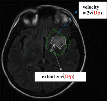

Fig. 31.2
The role of the product Dρ and the ratio D/ρ. The two contours come from the simulation of a patient case. The thick white contour corresponds to the threshold of cell density visible on MRI. The velocity of this visible tumor front is given by the formula 2√(Dρ). The dotted line is the contour corresponding to a cell density five times smaller than the threshold. The extent of the non-visible tumor part is tuned by the ratio D/ρ
More sophisticated tools are currently under development [12, 13], that will allow to estimate the optimized values of parameters minimizing the difference between real and simulated time series of segmented contours. This inverse problem is numerically highly challenging and even not always solvable given the paucity of datas (patients undergo usually two or three MRIs before treatment). At best, one can identify the two products ρDw and ρDg, Dw and Dg being the diffusion coefficients in white and grey matter respectively [13]. From this latter study, one can conclude that image-based model personalization will not be achievable in clinical practice, unless one can find an imaging modality that would be indicative of cell density. In this spirit, some authors proposed a method in contrast-enhancing DLGG, assuming that T1-gado and Flair contours correspond to two isolines of distinct visibility thresholds of cell density. They used the two-thresholds method for estimating the ratio D/ρ [14] and the aforementioned method of velocity of diameter expansion to compute the product Dρ. Their results will be discussed in the next paragraph, but it should be kept in mind that there is no evidence that T1-gado and Flair contours are correlated with distinct levels of cell density.
Finally, any image-based personalization implies the segmentations of the tumor on successive images, which is a time consuming task. Hence, this method should be combined in the future with automated tools of segmentation.
31.2.4 Parameters Values for DLGG
For low-grade glioma, values for parameters were initially extrapolated from the values found for high grade glioma and expected to be centered around 0.438/year for ρ and around 4.75 mm2/year for D [1]. A range of values has been proposed by Harpold et al. [15], with ρ between 1 and 10/year and D between 10 and 100 mm2/year. In a paper aiming to estimate the individual tumoral birthdates in a large series of DLGG glioma, a range of values for ρ and D was found, which significantly differed from the one previously proposed [16]. A first paper attempted to estimate D and ρ by eyeball fitting of a real patient evolution with simulated images. The best fit was achieved for the values ρ = 0.438/year and D = 3.65 mm2/year [6], which lies within the domain found by Gerin et al. A very recent study estimated D and ρ on a series of 14 patients with DLGG showing an area of contrast enhancement by using the two-threshold method [17]. While some of the values fall between the expected range, some others were more suggestive of a grade III, as it could have been anticipated given the presence of a contrast enhanced area. All results are summarized on the log-log plot on Fig. 31.3.
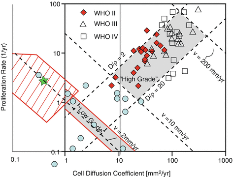

Fig. 31.3
Numerical values of D and ρ in a log-log plot. This diagram has been first discussed by Harpold et al. [15]. The diagonal v = 2 mm/year corresponds to those glioma with a constant product Dρ, with a VDE of 4 mm/year, which is the average value for DLGG. Red diamonds correspond to the values found by Ellingson et al. [20] for WHO grade II glioma. Their values are probably irrelevant, as they fall within the expected range for high-grade glioma. The values found by Gerin et al. [16] in the red dashed area are correctly centered around the diagonal with a VDE equal to 4 mm/year (i.e. v = 2 mm/year), but with values of the ratio D/ρ smaller than predicted by Harpold et al. Note that the green star, corresponding to the DLGG simulation performed by Jbabdi et al. [6], falls within the values found by Gerin et al. The blue circles correspond to values found in DLGG with contrast enhancement [17]
For the anisotropic version of the equation, it has been found that the ratio r of anisotropy of the tensor cells has to be increased about ten fold compared to the anisotropy given by the tensor of water diffusion measured on DTI, reflecting the well known propensity of glioma cells to migrate longitudinally rather than orthogonally to the axonal pathways [6]. This value was indeed needed to reproduce finely the shape of the tumor (which was known to be correlated with the shape of the white matter fasciculus [18]).
31.2.5 Virtual Imaging: Seeing Beyond the Visible
Interestingly, the ratio D/ρ controls the extent of non-visible part of the tumor (i.e. the number of cells located in areas with a cell density lower than the visibility threshold): the higher the ratio D/ρ, the greater the radiologically non-visible part of the tumor [19] (see Fig. 31.3). Although such virtual imaging could be potentially powerful, its practical interest is currently limited, for the two previously mentioned reasons: the lack of reliability of the visibility threshold hypothesis, and the challenging problem of determining the personalized values of ρ and D for each patient. Should such limitations be overcome, important applications would result, for surgical decision making and for designing radiation therapy margins.
31.3 Future Methods of Model Personalization
31.3.1 Apparent Diffusion Coefficient: The Missing Link Between MRI and Cell Density?
Ellingson et al. proposed in 2011 an elegant and powerful method to estimate 3D individual maps of proliferation and diffusion parameters from at least three longitudinal diffusion weighted sequences [20]. The key assumption is an inverse linear correlation between ADC and cell density (ADC = αc + β, α being negative). These authors have indeed found a negative correlation between cell density and apparent diffusion coefficient, measured from diffusion weighted sequences [21]. Assuming this relation, one can fully inverse the proliferation-diffusion equation, with ρ(x) and D(x) as the unknown variables (ρ(x) and D(x) are the proliferation and diffusion coefficient, that can vary with position x). Three successive ADC maps are nevertheless required, to estimate the time derivatives terms in the equation. The results give nice color maps for proliferation and diffusion, showing spatial changes of these parameters. However, the link between cell density and ADC is not that clear, as ADC changes can be observed in relation to demyelination, edema, and disruption of normal brain architecture [22, 23]. This might explain why the values found by these authors for ρ and D in low-grade glioma are not consistent with the values estimated by the aforementioned approach based on longitudinal morphological follow-up (see Fig. 31.3).
31.3.2 Towards Integration of Longitudinal Multimodality Imaging in the Model
Spectroscopic magnetic resonance imaging also offers a means to estimate cell density and/or proliferation rate of a DLGG, and to get a rough estimate of their spatial variations using multivoxels techniques [24, 25]. Similarly, indices derived from DTI sequences (p and q values, fiber density, …) could also be linked to the cell density in the invasion part outside the flair hypersignal. Hence, this information could potentially be used as inputs for the model personalization process. Promising methods, using a Bayesian framework, are under development to integrate these multimodality imaging and to manage the uncertainty inherent to these experimental data [26]. However, the key point in these methods still relies on the mathematical links between cell density and multimodal imaging parameters (ADC, Cho/NAA, CNI, p & q in DTI, …), and more efforts should be devoted to their determination.
31.4 Future Applications of Personalized Models
31.4.1 Model-Guided Optimization of Treatment Sequence
Assuming that the inverse problem has been solved—i.e. one is able to personalize the model based on (multimodal) MRI—treatment sequences can be simulated on the virtual tumor of the patient, allowing to select an optimized scheme for each patient. For example, it has been suggested that the benefit of gross total resection for tumors with high values of D/ρ is limited, since a lot of isolated tumor cells would be left even after a radiologically complete resection [27]. One study tested this idea in the context of glioblastoma, and found indeed in a large series of more than 200 patients that no survival benefit of complete resection versus biopsy was observed for patients with high values of D/ρ [28]. However, another study failed to replicate these results [14], proving that the personalization method (based on the hypothesis that T1-gado and Flair extent delineates two isolines of high and low cell density respectively) is not reliable (which does not come as a surprise, since it is well known that flair extent in glioblastoma may result from inflammatory or vasogenic edema, rather than from tumor cells only).
In the same vein, the model would predict that a supra-radical resection of high D/ρ tumors would dramatically increase the delay of recurrence [27]. Identifying these patients would be an essential step, as this information is another parameter to include in the evaluation of the onco-functional balance (see chapter on onco-functional balance by Mandonnet et al.).
Thus, the combined use of patient-specific simulations with tools of preoperative functionally-based prediction of extent of resection [29, 30] could assist the decision making process of surgery versus another oncological treatment (chemotherapy, radiation therapy). To this end, the effect of chemotherapy and radiation therapy should also be included in the model. Some attempts have already been done for modeling radiotherapy in high grade glioma [31, 32], but the validity of such models is not well established. Moreover, the prolonged effect of chemotherapy and radiation therapy in DLGG [33–35] warrants to develop specific models of DLGG response to these treatments [36, 37].
31.4.2 Model-Based Evaluation of Treatment Efficacy
The evaluation of treatment efficacy in DLGG is in itself a real challenge. The usual methodology of evidenced-based medicine that prevails in other fields of oncology, i.e. randomized studies comparing two treatment arms, is inadequate for DLGG (in their true low-grade period), given the very long survivals of these patients [38]. Moreover, most patients will ultimately also receive the treatment of the other arm, thus precluding to analyze separately the effect of each treatment. Personalized models can play an important role to quantify individual treatment response: for each patient, simulations can act as its own virtual control. Hence, response can be defined at any time as the difference between real (measured) tumor diameter in the patient under study and simulated (predicted) tumor diameter in its untreated virtual clone. In its simplified version, this method consists in comparing the slopes of tumor diameter growth curve before and during treatment.
31.4.3 The Backward Extrapolation
Simulations can also be used to estimate the real biological birthdate of a DLGG, which is anterior to the radiological birthdate estimated by a simple backward linear extrapolation (see chapter on dynamics of DLGG). It can be shown that, within some approximations of the proliferation-diffusion model, a corrective term of 20/v has to be added to the radiological birthdate [16], v being the velocity of diametric expansion (VDE). Applying this principles to a series of 144 patients, it has been found that patients could be classified roughly in two groups: a group of patients with low velocities (v between 1 and 4 mm/year) and a group with high velocities (v between 4 and 8 mm/year). For the low velocity group, patients are about 15 years of age at estimated biological onset, whereas for the high velocity group, patients ages are centered around 25 years of age [16]. Even if these results should be considered very cautiously given the strong underlying hypothesis of the model, they could help to identify different molecular signature of these two groups of tumors and to target age groups for a screening policy (see chapter screening).
Stay updated, free articles. Join our Telegram channel

Full access? Get Clinical Tree


